In this tutorial you can learn how superpositions can be created in a quantum circuit, how randomness affects quantum computations, and how interference can be detected in measurement results.
Prerequisite Tutorials:
• The Basics of Quantum Mechanics
• Quantum Algorithms & Quantum Circuits
Open the quantum circuit simulator in a separate window
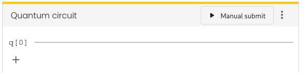
In this tutorial, we use only a single qubit. In the circuit simulator you can reduce the number of qubits by clicking the - button in the Quantum circuit box until only a single line with the qubit label q[0] is shown.
Simulation 1: Doing nothing
Let us start with the simplest quantum algorithm imaginable: The “do nothing algorithm”. It consists of the preparation of the qubit in the zero state $\ket{0}$ and its subsequent measurement, without any quantum gates in-between. As this is the default configuration of the circuit simulator, you do not have to do anything, i.e., the circuit should look like this:
Run the simulation several times by clicking the Manual submit button. Can you explain the observed probability distribution in the histogram? Do you find any randomness in the outcomes?
Explanation
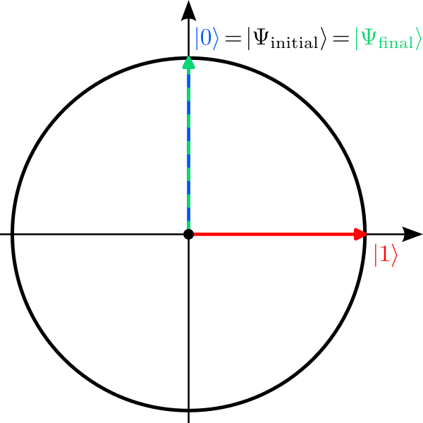
Without any gates, the transformation applied by the quantum computer is simply:
$$
\ket{\Psi_\mathrm{initial}}=\ket{0}
\;\xrightarrow{\; I \;}\;
\underbrace{1}_{\alpha}\ket{0}+\underbrace{0}_{\beta}\ket{1}
=\ket{\Psi_\mathrm{final}}
\;\xrightarrow{\mathrm{Measure}}\;
\begin{cases}\ket{0}&:\,p_0=1\\\ket{1}&:\,p_1=0\end{cases}
$$Here $I$ denotes the “do nothing operation” called identity. At the end the final state is measured and yields the result $\ket{0}$ with probability $p_0=1$. So in this example, the measurement outcome is indeed deterministic (but also very boring).
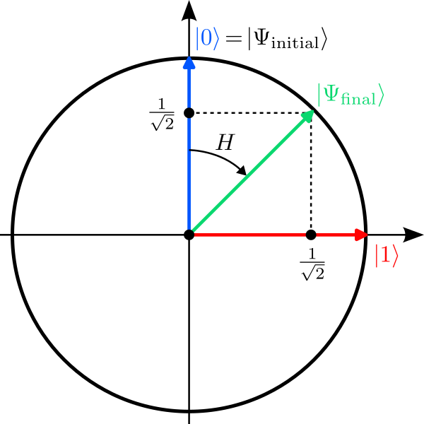
Simulation 2: Creating a superposition
Let us now create a superposition by applying a single Hadamard gate $H$ to our qubit. Its action on the two basis states of the qubit is defined as follows:$$
\begin{aligned}
\ket{0}\;&\xrightarrow{\;H\;}\;\frac{1}{\sqrt{2}}\ket{0}+\frac{1}{\sqrt{2}}\ket{1}\\
\ket{1}\;&\xrightarrow{\;H\;}\;\frac{1}{\sqrt{2}}\ket{0}-\frac{1}{\sqrt{2}}\ket{1}
\end{aligned}
$$Note that the vectors after the transformation have still length 1 since $\alpha^2+\beta^2=1$ in both cases! Geometrically, the Hadamard gate is the concatenation of two operations: A reflection about the y-axis followed by a clockwise 45° rotation about the origin.
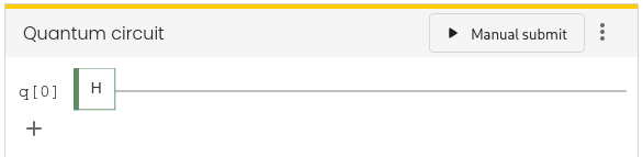
The Hadamard gate is represented by a square with the label H in the Gates box of the circuit simulator. Grab the box with your mouse and drop it onto the first line so that the gate is applied to the qubit with index 0. The circuit should look like this:
Run the simulation several times and observer how the results change with each run. Can you explain the observed probability distribution in the histogram?
Explanation
Applying a Hadamard gate $H$ to the qubit creates a superposition:
$$
\ket{\Psi_\mathrm{initial}}=\ket{0}
\;\xrightarrow{\; H \;}\;
\underbrace{\frac{1}{\sqrt{2}}}_{\alpha}\ket{0}+\underbrace{\frac{1}{\sqrt{2}}}_{\beta}\ket{1}=\ket{\Psi_\mathrm{final}}
\;\xrightarrow{\mathrm{Measure}}\;
\begin{cases}\ket{0}&:\,p_0=0.5\\\ket{1}&:\,p_1=0.5\end{cases}
$$In this case, we wittness the randomness of quantum mechanics for the first time: The qubit is measured in the state $\ket{0}$ with probability $p_0=\alpha^2=0.5$ and in the state $\ket{1}$ with probability $p_1=\beta^2=0.5$. The result you get from our simulator is based on $N=200$ shots, so that you can expect roughly $N_0\approx 100$ shots where the results was $\ket{0}$ and $N_1=N-N_0\approx 100$ where it was $\ket{1}$.
Simulation 3: Interference
One Hadamard gate creates a superposition with non-zero probability to find the qubit in the state $\ket{1}$. What happens if we apply a second Hadamard gate after the first one? Does the probability to find $\ket{1}$ increase further? Well, let’s try. Grab another H box and place it after the first one:
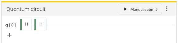
Run the simulation again several times and observer the histogram. Can you explain why the result is again deterministic and you never observe the state $\ket{1}$?
Explanation
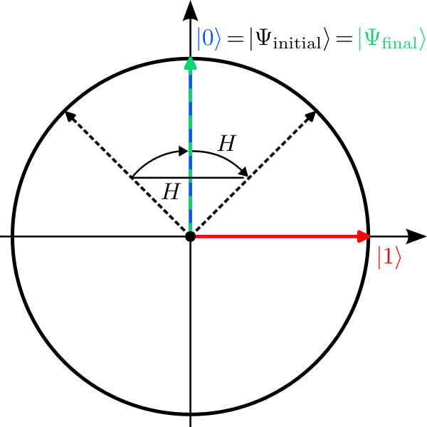
Applying two Hadamard gates $H$ transforms the qubit state as follows:
$$
\begin{aligned}
\ket{\Psi_\mathrm{initial}}=\ket{0}
\;&\xrightarrow{\; H \;}\;\frac{1}{\sqrt{2}}\ket{0}+\frac{1}{\sqrt{2}}\ket{1}
\\
&\;\xrightarrow{\; H \;}\;
\frac{1}{\sqrt{2}}\left(\frac{1}{\sqrt{2}}\ket{0}+\frac{1}{\sqrt{2}}\ket{1}\right)+\frac{1}{\sqrt{2}}\left(\frac{1}{\sqrt{2}}\ket{0}-\frac{1}{\sqrt{2}}\ket{1}\right)
\\
&\phantom{\;\xrightarrow{\; H \;}\;}=
\underbrace{\left(\frac{1}{2}+\frac{1}{2}\right)}_{\alpha}\,\ket{0}+\underbrace{\left(\frac{1}{2}-\frac{1}{2}\right)}_{\beta}\,\ket{1}
=\ket{\Psi_\mathrm{final}}
\\
&\;\xrightarrow{\mathrm{Measure}}\;
\begin{cases}\ket{0}&:\,p_0=1\\\ket{1}&:\,p_1=0\end{cases}
\end{aligned}
$$Here we had to use the rule how the Hadamard gate transforms the state $\ket{1}$. Note that the negative coefficient in this transformation precisely cancels the other term with $\ket{1}$, so that the final state has no contribution of $\ket{1}$ whatsoever. This cancelling of positive and negative amplitudes is called interference; it is one of the most important features for quantum algorithms. The final state after the application of two Hadamard gates is then just the initial state $\ket{\Psi_\mathrm{final}}=\ket{\Psi_\mathrm{initial}}=\ket{0}$ and we measure the qubit in state $\ket{0}$ with probability $p_0=1$.
Ⓒ2023 Tutorial by Nicolai Lang, Institute for Theoretical Physics III, University of Stuttgart