In this tutorial you can learn what a qubit is, why qubits can be in superposition states, where the randomness in quantum mechanics enters, and why quantum computers can do things that classical computers cannot.
This tutorial provides the necessary knowledge to understand all other tutorials and to use our interactive quantum circuit simulator to run simple quantum algorithms on our servers.
Prerequisite Tutorials:
None
Prerequisites
This primer on quantum mechanics & quantum computing targets a general audience with high school equivalent background in physics & mathematics. No academic degree required!
If you have learned about the following concepts, you are ready to go:
- Vectors
- Probabilities
- Trigonometry
- Complex numbers (optional)
The mathematical tools needed to understand and apply quantum mechanics are actually not too complicated. To provide perspective: All required mathematical concepts are taught in the first two semester of a typical study program in physics, mathematics, and even informatics or engineering. Quantum mechanics draws heavily from both analysis (integrals, differential equations, …) and linear algebra (vectors, inner products, linear maps, …). To describe quantum computers on an abstract level (to write “quantum programs”) linear algebra is even sufficient.
Reminder:
Meta-Knowledge
As a layperson (in this context: non-physicists), it is often hard to assess the status of scientific statements: are we talking about speculations, hypotheses, widely accepted theories, or well-tested observations? This “knowledge about knowledge” or “meta-knowledge” is just as important as the knowledge itself. To prevent misconceptions in this regard, here a few “meta-knowledge” facts about the knowledge you can learn in this tutorial:
- The tenets of quantum mechanics, with all their quirks and counterintuitive phenomena, are by now a well-established, extensively tested theory. This is as good as it gets in science. The formalism explained in this tutorial is learned (in a more mathematical fashion) by every undergrad of physics around the globe, just as you learn adding and multiplying numbers at school. From a physicist’s perspective, quantum mechanics is not a fancy or “esoteric” field of study (it is certainly interesting, though). This also means that none of the predictions of quantum mechanics presented here are hypothetical. All of them have been experimentally tested repeatedly. Seemingly “strange” quantum phenomena like superpositions, entanglement, quantum “teleportation”, etc., are by now standard tools in laboratories (some even in advanced lab courses and/or commercial devices). Creating entangled pairs of photons is for an experimental quantum physicist like mixing a salad dressing is for a professional chef: It’s nice that you can produce them, it is certainly useful for your job, but it’s nothing to be excited about.
- Since the predictions based on quantum mechanical laws (in their precise mathematical form) perfectly match experiments, we trust these equations like engineers trusts the laws of classical mechanics to construct airplanes. Consequently, we can use them to engineer “quantum machines” like a quantum computer. So if you ask how a specific quantum phenomenon can be theoretically modeled and explained, you most likely will be given a precise answer.
- The situation is very different if, instead of how, you ask why a certain phenomenon is the way it is. The question why entanglement exists in our universe, and why quantum mechanics is a probabilistic theory, are important and deep questions that should be asked. You will not find answers to these questions here because, as of now, there is no consensus among physicists what the correct answers are. There are hypotheses, untested theories, that draw rough pictures of what quantum mechanics might tell us about reality — but none of them are clearly backed by experiments. In this sense, quantum mechanics is a highly useful theory as it stands, but it might be expanded into another, deeper theory in the future. This does not mean that quantum mechanics is potentially wrong (it is not, it works perfectly in our experiments!). It only means that its range of validity may be restricted; just as Newtonian mechanics has not been “proven wrong” by Einstein’s general theory of relativity (it is the limit of Einstein’s theory for small velocities and small masses.). The bottom line is: There is still fundamental work to be done and new features of our world are waiting to be discovered, but quantum mechanics, as we teach and use it today, will never lose its merits.
- Luckily, an engineer does not need to know a deeper reason for gravity (like the general theory of relativity) to build an airplane; understanding the laws of classical mechanics is completely sufficient. For the same reason, we are not hindered by the fact that we cannot explain why quantum mechanics is the way it is on our quest to build a quantum computer.
From Vectors to Qubits
Note for experts:
In this tutorial we restrict amplitudes to real numbers instead of complex numbers to make it accessible for high school students.
We comment on the role of complex numbers at the end.
Qubits are the elementary carriers of information of a quantum computer. They play the same role as the bits stored on the hard drive of your notebook which are processed by its central processing unit (CPU) to make fun stuff happen (like printing these letters on your screen). Similarly, a quantum computer must be able to store qubits on a “quantum hard drive” (this is called a quantum memory) and to manipulate qubits on some sort of “quantum CPU” (a quantum processor). The goal of the QRydDemo project is to build such a quantum processor, where each qubit is encoded by a single atom and the manipulations are done by hitting these atoms with lasers (see Platform for more details).
When you think about the bits whizzing around in your notebook, you typically do this in an abstract way: they are just “things” with two possible states (1 or 0); you completely ignore what exactly these two states are (like: high/low voltage in wires, or up/down magnetization on the disc of a hard drive). Why? Because it is a useful abstraction for writing programs! The same is true for programming quantum computers: While the “quantum engineers” (that’s us) who build a quantum processor must be aware of how the qubits are implemented, the “quantum programmer” who uses the quantum computer to run “quantum software” can safely ignore these details and think of qubits as abstract pieces of quantum information. In the following, we will speak about qubits and the things we can do with them in this abstract way. This abstract level to talk about quantum mechanical systems is called quantum information theory.
But what is a qubit, abstractly speaking? One often hears that “a qubit is like a classical bit that can be 0 and 1 at the same time” – but what does that actually mean? Whenever words are too vague to explain things, mathematics comes to the rescue:
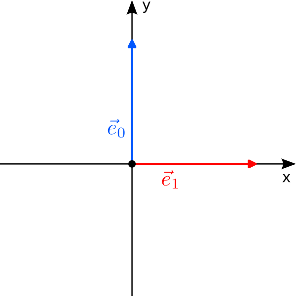
Let us start with a fancy classical bit. Instead of “0” and “1”, we use the two orthogonal vectors$$
0\leftrightarrow\vec e_0 = \begin{pmatrix} 0\\1\end{pmatrix}
\qquad\text{and}\qquad
1\leftrightarrow\vec e_1 = \begin{pmatrix}1\\0\end{pmatrix}
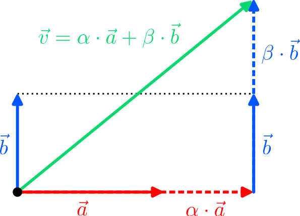
$$ to label the two states of the bit. There are two immediate questions: Why are we allowed to do this, and why should we do it? The answer to the first question is simple: “0” and “1” are just labels to refer to two states of a system, and we are free to choose different labels, for instance $\vec e_0$ and $\vec e_1$. However, just because we can doesn’t mean we should; and writing $\vec e_0$ is clearly more cumbersome than “0”. But remember that we would like to come up with a thing that can be in two states at once. There is no natural way to combine the discrete states “0” and “1” to something “in between”; but there is for vectors: We can scale and add vectors to form new vectors, a procedure called linear combination!
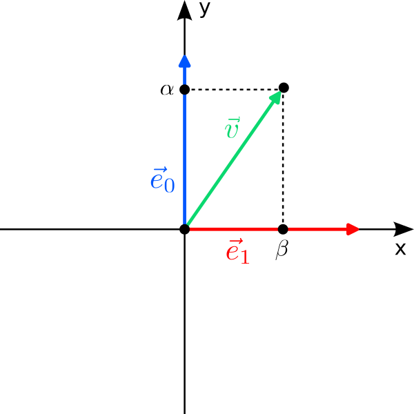
The most general linear combination of our two “bit vectors” is the vector
$$
\vec v =\alpha\cdot\vec e_0+\beta\cdot\vec e_1=
\begin{pmatrix} \beta\\\alpha\end{pmatrix}
$$ with arbitrary real coefficients $\alpha,\beta\in\mathbb{R}$ that are called amplitudes in quantum mechanics. For $\alpha=1$ and $\beta=0$ it is $\vec v = \vec e_0$ (the “0”), while for $\alpha=0$ and $\beta=1$ it is $\vec v=\vec e_1$ (the “1”). But for, say, $\alpha =0.2$ and $\beta=-0.8$, $\vec v$ is neither $\vec e_0$ nor $\vec e_1$; it is as if $\vec v$ has a bit of both $\vec e_0$ and $\vec e_1$ at the same time! We can therefore put forward the following hypothesis:
The state of a single qubit is described by a two-dimensional vector $\vec v$.
This is correct, but we missed one point. The vector that describes the state of a qubit must have length 1 (in mathematics one calls such vectors normalized):$$
|\vec v |=\sqrt{\alpha^2+\beta^2}\stackrel{!}{=}1
$$Why, you ask? Well, this has to do with what happens if we “look” at the qubit, a process called measurement. We will discuss the important role of measurements in quantum mechanics in the next section. Before that, let us briefly digress and have a look at how we actually realize qubits at the QRydDemo project.
To realize a qubit in the laboratory, one needs a system with two internal states that are then labeled by $\vec e_0$ and $\vec e_1$. At the QRydDemo project, we use single Strontium atoms to realize qubits. (Strontium is an alkaline earth metal that is responsible for the red colors of fireworks.) These Strontium atoms are cooled down and then trapped by lasers in an evacuated glass chamber. We can use the lasers like “tweezers” to trap and arrange Strontium atoms in almost arbitrary patterns. If we illuminate these atoms with another laser of a specific wavelength (= color), the atoms start to glow (they fluoresce). This glowing can be detected by a very sensitive digital camera that observes the trapped atoms through a microscope. A photograph of 10 atoms arranged in a chain looks like this:
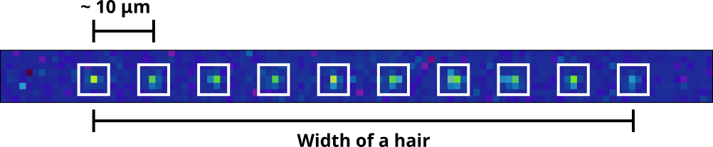
The white boxes are drawn on top of the image to mark the position of the atoms, so that we know their location even when they are not excited by a laser (they are then dark and invisible). And yes, every glowing blob in the above photograph is a single atom.
Each of these atoms is used to realize a qubit. But what are the two states? From chemistry you know that the electrons of an atom all live in a discrete set of orbitals. Orbitals look like strangely shaped clouds around the nucleus of the atom, and their density tells you the probability to find an electron at that position. Orbitals are the quantum mechanically correct description of the energy levels in the simpler (and outdated) Bohr model. Their existence and shape are a direct consequence of quantum mechanics, but here we simply want to use them as our two states! Thus we pick two specific orbitals of Strontium, let us call them $A$ and $B$; these orbitals describe the quantum state of the electrons that make up the atomic shell of Strontium:
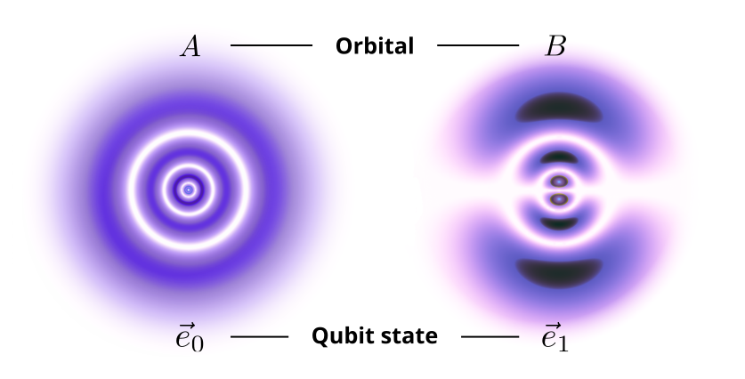
An atom with electrons in orbital $A$ then corresponds to a qubit in state $\vec e_0$, whereas an atom with electrons in orbital $B$ corresponds to the qubit state $\vec e_1$. Because the electrons are governed by quantum mechanics, the state of a Strontium atom can also be in a linear combination of $\vec e_0$ and $\vec e_1$, i.e., a superposition state.
Now you know how we realize qubits in our laboratory. But why single atoms, you might ask? Isn’t it very complicated to work with single atoms? (It is!) Why not larger objects that are easier to control? This is a good question and it has to do with our next topic: measurements. You will see below that in quantum mechanics obtaining information about the state of a qubit changes the state itself. But this means that if something (say, an air molecule or a single photon) bumps into your qubit and carries away information about its state, this interaction perturbs the qubit. For a qubit to be useful, one must therefore be able to shield it almost perfectly from all possible environmental influences. This shielding is much easier for atoms in vacuum than for larger (“macroscopic”) objects that very easily spread information about their state into the environment. So yes, controlling single atoms is hard, but we are rewarded with qubits that preserve their quantum states long enough so that one can hope to do useful computations with them.
Let us now return to our abstract description of qubits and discuss how measurements are described in quantum mechanics.
- The state of a qubit is described by a two-dimensional vector of length one. A qubit is not a classical bit that is in an unkown state 0 or 1.
- The state vector can be constructed as a linear combination of two orthogonal basis vectors; these linear combinations are called superpositions.
- The components of the vector are called amplitudes and can be negative. Their potential negativity is a crucial feature of quantum mechanics and allows for interference, a phenomenon that underlies the speedup of quantum computers.
- The QRydDemo project realizes qubits by single Strontium atoms that are trapped by lasers. The states of a qubit correspond to the states of the electrons in the shell of a Strontium atom.
Beware:
The vector $\vec v\in\mathbb{R}^2$ is not a vector in real space, like, e.g., the accelaration vector $\vec a$ of a particle. It is an abstract pair of real numbers that describes the state of a system, rather like the pair $(P,T)$ of pressure $P$ and temperature $T$ describes the property of the air in your room.
Beware:
The glowing blobs in the photograph of 10 atoms stretch over several pixels and give the impression of being “out of focus”. They look a bit like a distant planet viewed through a cheap telescope. This analogy is misleading! If you use a better telescope, the image of a planet becomes sharper and more resolved; eventually, you’ll see its pole caps, mountains and valleys. No matter how good our microscope and our camera are, the blobs will never become “sharp” and show you how an atom really “looks like”. Strontium atoms have a diameter of roughly 0.1 nanometer. The light we use to make the photograph has a wavelength of roughly 500 nanometer! It does not make sense to ask how something “looks to the eye” on this scale. It doesn’t look like anything!
Let that sink in.
Measurements
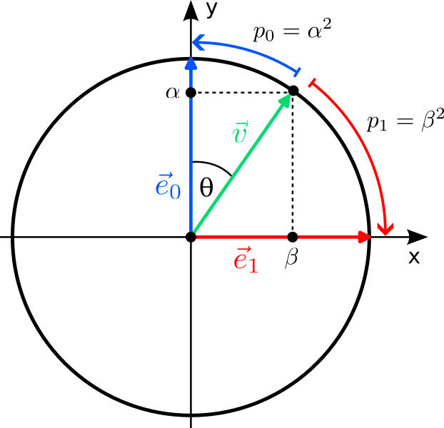
If you think about it, our hypothesis that the state of a qubit is described by a two-dimensional vector $\vec v$ isn’t very “quantum”. After all, there are many classical systems that can be described by two-dimensional vectors: The direction and strength in which the wind blows or the magnetic field of the earth points to can both be described in this way — and there is nothing “quantum” about them. To put it differently: So far our qubit seems to be a bit like a little compass needle that can point in different directions $\vec v$. The quantumness enters the stage when we measure the qubit. In classical physics, there is a one-to-one correspondence between states and observations: Systems in different states look differently when we measure them. At first, this statement seems tautological: isn’t it the sole purpose of different states to describe the different observations we can make? In classical physics, yes; in quantum mechanics, no! When you measure a qubit, it does not look like a compass needle pointing in the direction $\vec v$; it looks like a classical bit pointing in either $\vec e_0$ or $\vec e_1$ and nothing in-between. The probabilities of either result depend on the state $\vec v$, and, as it turns out, are given by the squares of the amplitudes of the vector:
$$
\vec v = \alpha\,\vec e_0+\beta\,\vec e_1
\;\xrightarrow{\;\text{Measurement}\;}\;
\vec v_\mathrm{new}=\begin{cases}
\vec e_0 &\text{with probability}\; p_0=\alpha^2\\
\vec e_1 &\text{with probability}\; p_1=\beta^2\\
\end{cases}
$$Here, $\vec v_\mathrm{new}$ denotes the new state of the qubit after the measurement.
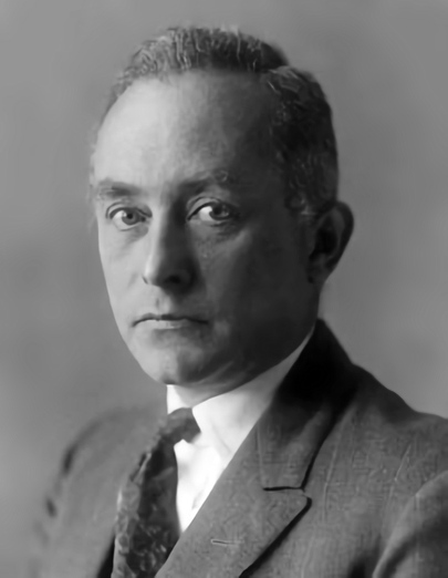
This rule, which has been confirmed by hundreds of quantum mechanical experiments by now, was formulated by the physicist Max Born and is thus called the Born rule. Let us highlight the three important (and unintuitive!) features of a quantum mechanical measurement:
- The outcome of the measurement is discrete (either $\vec e_0$ or $\vec e_1$) although the quantum state $\vec v$ can point in any direction (= is continuous). This emergent discreteness is called quantization and responsible for the name “quantum” in “quantum mechanics”.
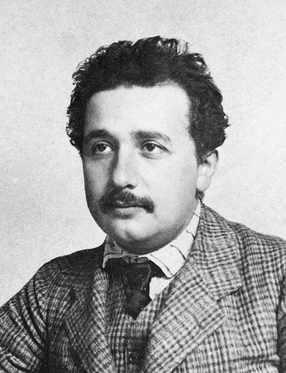
- The measurement outcomes are probabilistic: $\vec e_0$ and $\vec e_1$ are measured randomly with probabilities $p_0$ and $p_1$ (which depend on $\vec v$). This is the famous randomness of quantum mechanics which Albert Einstein didn’t like (see below).
- The quantum state is changed by the measurement, i.e., the state changes from $\vec v$ to either $\vec e_0$ or $\vec e_1$, depending on the measurement outcome. In quantum mechanics, measurements are thus not passive observations (like in classical physics), but affect the system that is observed! This phenomenon is known as wave function collapse.
The Born rule also explains why the vector $\vec v$ must have length 1: Probabilities must add up to 1, and because we interpret the squares of the coefficients as probabilities, they also must add up to 1; but this sum is nothing but the length of $\vec v$ squared:$$
p_0+p_1\stackrel{!}{=}1
\quad\Leftrightarrow\quad
|\vec v|^2=\alpha^2+\beta^2\stackrel{!}{=}1
\quad\Leftrightarrow\quad
|\vec v|\stackrel{!}{=}1
$$
There is a very convenient way to parametrize such vectors: They correspond exactly to the points on a circle of radius 1 (a unit circle). But a point on the circle can be described by a single angle $\theta$, where the components (amplitudes) of the vector are given by the two trigonometric functions sine and cosine:
$$
\vec v =\cos(\theta)\,\vec e_0+\sin(\theta)\,\vec e_1=
\begin{pmatrix}\sin(\theta)\\\cos(\theta)\end{pmatrix}
\quad\text{for}\quad 0\leq \theta < 2\pi
$$This vector is automatically normalized for all $\theta$ because $\sin^2(\theta)+\cos^2(\theta)=1$. So one should think of the set of all states of a qubit as a circle, where states closer to the x axis are more likely to be measured in $\vec e_1$, and states closer to the y axis more likely collapse to $\vec e_0$. The “set of all states” is refered to as a state space in physics.
Let us summarize what we learned so far:
The state of a single qubit is described by a two-dimensional vector$$
\vec v=\begin{pmatrix}\beta\\\alpha\end{pmatrix}
$$ of length $|\vec v|=\sqrt{\alpha^2+\beta^2}=1$.
If the qubit is measured, it is found either in state$$
\vec e_0=\begin{pmatrix}0\\1\end{pmatrix}
$$with probability $p_0=\alpha^2$, or in state$$
\vec e_1=\begin{pmatrix}1\\0\end{pmatrix}
$$with probability $p_1=\beta^2$.
The measurement changes the state of the qubit and is probabilistic.
The change of the qubit state by measuring it — the wave function collapse — is a fundamental principle of quantum mechanics. The fact that the outcome is undetermined until the measurement is performed (and only probabilities can be predicted) makes quantum mechanics an inherently probabilistic theory, a fact that vexed Albert Einstein who exclaimed that “God does not play dice […].” However, in the days since Einstein, experiments of physicists all over the world repeatedly confirmed the predictions of quantum mechanics, and clearly indicate that nature is somewhat of a gambling addict. To fathom the philosophical ramifications of the probabilistic measurement outcomes completely, one must be very clear about the type of randomness we are talking about: If you put a coin in a cup, shake, and put the cup upside down on the table, you have no clue whether the coin landed head or tail until you lift the cup and look. You could say the coin is like a qubit in that you can only predict the probabilities of head and tail when lifting the cup. This analogy is false, though! The difference is that although you do not know whether the coin landed head or tail when the cup hides it, the coin of course landed either head or tail. The probability just reflects your lack of knowledge of the real state of the coin (you could use the X-ray apparatus you happen to have beneath the table to look through the table and check this!). For all we know — and there are ingenious experiments known as Bell tests that support this — the probabilities predicted by quantum mechanics are not consequences of you, the observer, not knowing the “real” state of the qubit before a measurement. The “real” state of the qubit is $\vec v$ until you measure it; and by measuring it you actively change its state on the fly to either $\vec e_0$ or $\vec e_1$. This interpretation of quantum mechanics, known as Copenhagen interpretation, is the most widely held view among quantum physicists.
At the QRydDemo project, we are no philsophers of science, we are “quantum engineers” who want to build a quantum computer. But still we are affected by this inherent randomness: Whenever a quantum computer performs transformations on its qubits, we have to measure them at the end to extract the outcome of the algorithm. The results we get will be randomly distributed according to some probabilities. This means that quantum algorithms must be run several times (on the order of hundreds to thousands) so that all collected results can be averaged. These averages (which approximate the probabilities predicted by quantum mechanics) are then the real result of the quantum computation. The different runs of the same algorithm to collect data for the averaging are called “shots” in quantum computing parlance.
- Measurements in quantum mechanics are described by the Born rule according to which a qubit is measured in one of two discrete states with probabilies that equal the squares of the amplitudes of its state vector.
- State vectors must be normalized because we interpret the squares of their amplitudes as probabilities.
- Measurements in quantum mechanics modify the state of the object measured. This is called wave function collapse.
- The measurement process makes quantum mechanic a probabilistic theory. For quantum computing this implies that algorithms must be run several times to compute averages.
- The randomness of measurement outcomes is not due to a lack of knowledge of “hidden parameters”.
Beware:
Measuring is often sloppily referred to as “looking at” or “observing” the qubit. However, according to the standard interpretation of quantum mechanics, the measurement process does not have to involve a conscious being (like you) observing the qubit. A measurement in the quantum mechanical sense is any interaction that spreads information about the state of a system into its environment. For instance, pointing a laser at an atom and recording its state with a digital camera counts as measurement (even if you do not look at the taken picture). This also means that a single photon bumping into a qubit can set off an avalance of information about the qubit’s state that spreads into the environment. This makes the realization of qubits so hard because one must prevent these “accidental measurements” that collapse the qubit state at all costs.
There are alternative, less popular interpretations of quantum mechanics that predict the same outcomes as the Copenhagen interpretation but interpret the measurement process and the role of the quantum state differently. For example, hidden-variable theories and of course the quite famous Many-worlds interpretation.
Quantum physics notation
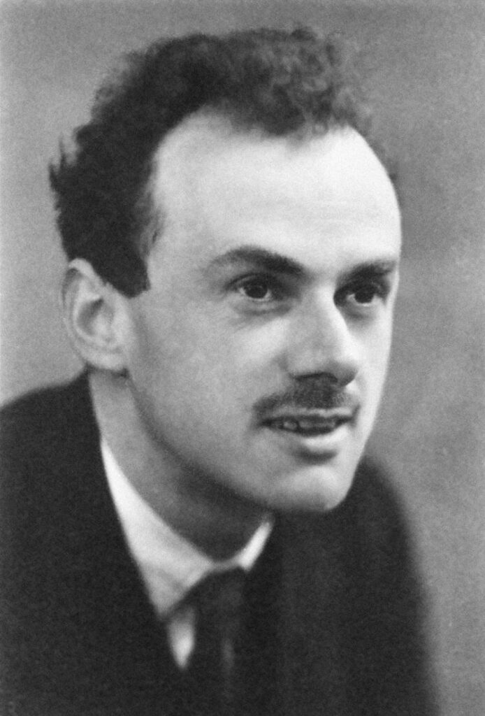
If you previously encountered a text on quantum mechanics, you may wonder why none of the above formula look familiar. The reason is that physicists (more precisely: Paul Dirac) invented a fancy notation for vectors:
$$
\vec v\rightarrow\ket{\Psi}
\quad\text{and}\quad
\vec e_0\rightarrow\ket{0}
\quad\text{and}\quad
\vec e_1\rightarrow\ket{1}
$$The linear combination above then looks like$$
\ket{\Psi}=\alpha\ket{0}+\beta\ket{1}
\qquad\text{with}\qquad \alpha^2+\beta^2=1
$$and is called the quantum state (or wave function) of a single qubit. The numbers $\alpha$ and $\beta$ describe the state completely and are called (probability) amplitudes. A vector of the form $\ket{…}$ is called a ket.
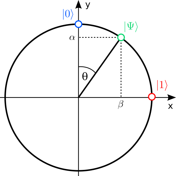
Rephrased in this new notation, a point on the unit circle describes the quantum state $\ket{\Psi}$ of a single qubit, and the unit vectors that define the two axes are $\ket{0}$ and $\ket{1}$. The projections of $\ket{\Psi}$ onto the axis are the amplitudes $\alpha$ and $\beta$.
To be fair: this change of notation is not just to make quantum mechanics “look fancy.” There is a deep mathematical reason why this is a very convenient notation, but this goes far beyond this tutorial. (The notation is called Dirac- or bra-ket notation; the mathematical reason is known as Riesz representation theorem and has to do with how inner products are calculated in this formalism.)
We will stick to this notation in the following because it makes it easy to generalize quantum states to many qubits.
Beware:
The terms “quantum state” and “wave function” are often used synonymously. The reason is that historically, the first quantum states described where a quantum mechanical particle is located in space. These quantum states are functions and typically have a wave-like nature, hence “wave functions”. The states $\ket{0}$ and $\ket{1}$ of our qubits do not describe their position, so that $\ket{\Psi}$ is neither a function nor a wave. We therefore stick to the term quantum state.
Many qubits
So far we only talked about a single qubit. Just as a computer that can store a single bit is useless, a quantum computer with a single qubit is nothing to be proud of. To make quantum computers shine, we need many qubits. Two questions come to mind immediately: How to describe the quantum state of many qubits, and how many is “many” to make a quantum computer useful?
Quantum states of many qubits
To answer the first question, we must let go of the possibility to visualize the different states many qubits can have; the image of a circle motivated above really only works for a single qubit. The mathematical formalism of linear combinations of vectors, however, carries over to as many qubits as we like. If we follow the concept of measurements in quantum mechanics, we should expect that if we measure $N$ qubits, we will observe a result that looks like $N$ bits, where each bit can be either in state “0” or in state “1”. We write such a quantum state (vector!) where $N$ qubits are in the configurations $x_i\in\{0,1\}$ ($i=1,2,\dots,N$ labels the qubits) as $$
\ket{x_1,x_2,\dots,x_N}=\ket{x_1x_2\dots x_N}\,.
$$In the last expression we dropped the commas to simplify the notation. We call these “classically looking” states basis states or basis vectors. How many such basis states are there?
Let us consider an example: If we have only $N=2$ qubits and measure them, we will find one of the $4=2^2$ states$$
\ket{00},\;\ket{01},\;\ket{10},\;\ket{11}\,.
$$Remember that for a single qubit the two states $\ket{0}$ and $\ket{1}$ were simply fancy names for two orthogonal vectors of length 1. The same is true for the four vectors above. But, you say, there are no more than 3 orthogonal vectors in our three-dimensional space, where does the fourth one point to? Well, you have been warned that one can no longer visualize the state space of many qubits. Now you know why: To describe the states for two qubits, one needs a four-dimensional space $\mathbb{R}^4$.
In general, there are $2^N$ possible configurations that $N$ bits can have, so that’s how many potential measurement outcomes a system of $N$ qubits has. Each corresponds to a vector $\ket{x_1x_2\dots x_N}$ that is orthogonal to all others, so that a $2^N$-dimensional space $\mathbb{R}^{(2^N)}$ is required to describe the quantum states of $N$ qubits. Remember that the state vector $\vec v$ (or $\ket{\Psi}$ in the new notation) is not a vector in our space, but a rather abstract “collection of numbers”. Thus there is nothing inherently problematic about higher-dimensional spaces to describe many qubits. The mathematics of linear algebra really doesn’t care how many dimensions you have. The only downside is that we can no longer imagine how a quantum state “looks like”. Fortunately, that’s the great strength (and beauty) of mathematics: Whether we can visualize something does not matter, we can always do abstract calculations with it!
The abstract expressions we are particularly interested in as quantum physicists are linear combinations, of course. After all, that is what quantum mechanics is all about. The most general linear combination of the four basis vectors for $N=2$ qubits is simply$$
\ket{\Psi}=\alpha\ket{00}+\beta\ket{01}+\gamma\ket{10}+\delta\ket{11}
$$where the four real numbers $\alpha,\beta,\gamma,\delta\in\mathbb{R}$ are our new amplitudes. Because two qubits can be observed in four different states, we now have just as many amplitudes (in general, the quantum state of $N$ qubits has $2^N$ amplitudes). The Born rule also generalizes in a straightforward way:$$
\ket{\Psi}
\;\xrightarrow{\;\text{Measurement}\;}\;
\ket{\Psi_\mathrm{new}}=\begin{cases}
\ket{00} &\text{with probability}\; p_0=\alpha^2\\
\ket{01} &\text{with probability}\; p_1=\beta^2\\
\ket{10} &\text{with probability}\; p_2=\gamma^2\\
\ket{11} &\text{with probability}\; p_3=\delta^2\\
\end{cases}
$$The probabilities are again given by the squares of the amplitudes. Since the four probabilities must add up to 1, the “normalization constraint” is now$$
\alpha^2+\beta^2+\gamma^2+\delta^2\stackrel{!}{=}1\,.
$$In the four dimensional space $\mathbb{R}^4$ to which $\ket{\Psi}$ belongs, this is still equivalent to the requirement that $\ket{\Psi}$ has length 1 (= is normalized). So once we let go of our desire to visualize states and embrace abstract mathematics, there is actually not that much new about the quantum states of many qubits.
Before we proceed with answering how many qubits we need, let us digress and see how we measure a many-qubit quantum state on the QRydDemo platform. Recall that our qubits are encoded in the electronic states (orbitals) of single Strontium atoms, each trapped by a laser at a fixed position. The two orbitals $A$ and $B$ we chose to represent the qubit states $\ket{0}$ and $\ket{1}$ have the nice property that only atoms in orbital $B$ (= state $\ket{1}$) respond to laser light of a specific wavelength. “Responding” means that atoms in state $\ket{1}$ fluoresce, i.e., they glow if we take a picture. If we draw a square where we know an atom must be trapped, a measurement of a multi-qubit state is performed by illuminating all atoms with the laser, and recording with the camera which atom glows and which remains dark:
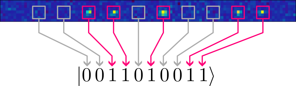
We can then read off the measured state by checking the boxes: dark boxes correspond to a qubit in state $\ket{0}$, boxes with a glowing blob to a qubit in state $\ket{1}$. In the example above we measured the 10-qubit state $\ket{\Psi}=\ket{0011010011}$.
- When measured, $N$ qubits can be observed in the $2^N$ possible configurations of $N$ classical bits.
- Each outcome is described by a normalized vector that is orthogonal to all other outcome vectors. A general quantum state of $N$ qubits is therefore a linear combination of these $2^N$ vectors and belongs to a
$2^N$-dimensional vector space. - The quantum state of $N>1$ qubits cannot be visualized in our three-dimensional world.
- The quantum state of $N$ qubits is completely specified by its $2^N$ real amplitudes.
- The Born rule generalizes to many qubits. The probabilities for measurement outcomes are still given by the squares of the corresponding amplitudes.
- On the QRydDemo platform, we measure the quantum state of many qubits with a laser of a specific wavelength. Strontium atoms in state $\ket{1}$ glow, whereas atoms in state $\ket{0}$ remain dark.
Beware:
One might be tempted to think of the state of $N$ qubits being somehow described by $N$ points on a unit circle, where the position of each point describes the state of one of the qubits. That this is not the case follows from a simple counting argument: We need $2^N$ real numbers (= amplitudes) to describe a $N$ qubit quantum state, but only $N$ real numbers (= angles) are needed to describe $N$ points on a unit circle. Since $2^N>N$, the picture of a unit circle lacks a lot of “degrees of freedom” and is therefore wrong.
How many is “many”?
Now that we know what a “many-qubit quantum state” looks like (abstractly and in reality!), we can finally answer the second question, namely how many qubits are needed to make a quantum computer useful. To this end, let us assume we have a classical computer (right now that’s all we have anyway) and would like to simulate how the quantum state of $N$ qubits evolves over time; for instance, we would like to simulate a quantum computer! To do this, we have to store the quantum state somehow. But knowing the quantum state is tantamount to knowing all amplitudes $\alpha,\beta,\dots$. Each amplitude is a real number that we can store in our classical computer approximately. In a programming language we would use a variable for this purpose for which your computer typically reserves 4 bytes of your random access memory (RAM). How much memory $M$ do we need to store all amplitudes of the quantum state of $N$ qubits? Easy:$$
M=2^N\times 4\,\mathrm{byte}\,.
$$So for 2 qubits we need as little as $M=16\,\text{byte}$ of memory. How much qubits do you think you can simulate on your computer that has, let’s say, around $M=16\,\mathrm{Gigabyte}$ of RAM? Well:$$
N=\log_{2}(M/4\,\mathrm{byte})=\log_{2}(16\cdot 10^9/4)\approx 32
$$That’s not very impressive. Remember that for us at the QRydDemo project a single qubit is realized by a single atom. So we only need 32 atoms to realize as many qubits! At our institutes we have of course specialized computers to do such simulations. They have up to $M=1\,\mathrm{Terabyte}=1000\,\mathrm{Gigabyte}$ of RAM (and cost up to 10.000€!). So let’s see how many qubits we can simulate on our specialized hardware:$$
N=\log_{2}(M/4\,\mathrm{byte})=\log_{2}(1000\cdot 10^9/4)\approx 38
$$Ouch! With our very expensive computers we can simulate only 6 qubits more than you! This is of course embarassing, and by now you certainly figured out what’s going on: The number of amplitudes that define a quantum state, and therefore the amount of memory needed to simulate such a state on a classical computer, grows (better: explodes) exponentially with the number of qubits. While a quantum computer with $N=100$ qubits (= atoms) is perfectly conceivable (that’s actually our first goal for our QRydDemo quantum processor), simulating such a machine on a classical computer would require$$
M=2^{100}\times 4\,\mathrm{byte}=5070602400912917605\,\mathrm{Terabyte}
$$of memory. It should be clear that a classical computer with that much memory will never exist (and no, Moore’s Law will not save us).
We have learned an important lesson: A machine that can store and manipulate around $N\sim 100$ qubits in a controlled fashion — let us call such a machine a quantum computer — cannot be simulated on any classical computer that we will ever possess. So whatever the outputs (= measurement results) of such a quantum machine are, we have no chance to predict them by simulating it on a classical computer. If we want to know the results, we have only one choice: Build the quantum machine! This is the reason why we (and many others) are trying to build a quantum computer with $N\gtrsim 100$ qubits (actually $N\gtrsim 50$ would already be a big win, just do the math and try to find a computer with that much memory).
The next question is of course why we sould be interested in the outputs of such a quantum machine in the first place? Just because a result is hard to compute doesn’t make it useful. What are the tasks that make a quantum computer shine?
- Because the number of amplitudes to describe a quantum state of many qubits is exponentially large in the number of qubits, storing the quantum state of 100 qubits already requires roughly 1018 Terabyte of storage on a classical computer.
- Therefore classical computers cannot be used to simulate quantum systems with many degrees of freedom (e.g. many electrons).
- By contrast, quantum computers can simulate quantum mechanical systems much faster than classical computers.
- The capabilities of a quantum computer with about 100 qubits is already far beyond anything we can (and will ever) simulate on a classical computer.
- While quantum computers can speed up classical problems like integer factorization and database queries, their most important application is the speedup of quantum mechanical simulations, e.g., for drug development and materials science.
Beware:
In our counting of qubits we assumed that these qubits are “perfect”, i.e., not affected by noise. In reality, this is almost impossible to achieve, which is why one has to “merge” several of these noisy “physical” qubits to form a robust “logical” qubit. This procedure is known as quantum error correction and blows up the number of (physical) qubits considerably. This is one of the reasons why building a full-fledged quantum computer is so hard.
What are quantum computers good at?
Quantum computers are good at manipulating qubits without having to store their amplitudes like a classical computer. To store the quantum state of 100 qubits on the QRydDemo platform, we need, well, 100 qubits. Since every qubit is realized by a single Strontium atom, we only require 100 atoms to encode and manipulate a quantum state that, on a classical computer, would require more memory than we can imagine. That’s why quantum computers are so fascinating: they can store and manipulate quantum states without having to pay with staggering amounts of memory like classical computers.
If we take a step back, we catched a glimpse of a much deeper insight:
Quantum computers are good at simulating quantum mechanics.
The first who pointed this out was the famous physicist Richard Feynman who advertised quantum computers as efficient simulators for quantum mechanics, today known as (digital) quantum simulators.
This statement seems tautological. It sounds like “a classical computer is good at simulating electronic circuits”. True! But we also learned that:
Classical computers are really bad at simulating quantum mechanics.
Unfortunately, we know that our world, at the deepest levels, is governed by quantum mechanics. For example, the Standard Model of particle physics that describes quarks and electrons and the like is a quantum mechanical model. And if we want to compute it’s predictions to compare them to measurements made at particle colliders like CERN we somehow must “simulate the theory”, i.e., evaluate its predictions. But this is hard (or even impossible) on classical computers as we just learned. Another example is the simulation of materials like high temperature superconductors (which are used in MRI scanners); their strange (and useful) feature of superconductivity is an effect of many interacting electrons — which are governed by quantum mechanics! Again, physicists have a really hard time to understand (and design) these materials because we would need a machine that can simulate quantum mechanics. We would need a quantum computer! You could also ask why chemists, who develop novel drugs or more efficient solar cells, have to perform expensive and time consuming trial-and-error experiments. Chemistry is, after all, “just” applied quantum mechanics: when you trigger a chemical reaction where electrons and nuclei form new molecules, the equations of quantum mechanics should (and could) tell us what the result will be and which properties it has. Why bother with experiments? Well, because we cannot solve the equations for the very reason explained above: too many amplitudes! A quantum computer could simulate these reactions and considerably speed up materials science.
At this point you may wonder: Wait, isn’t the “killer application” of a quantum computer the famous Shor algorithm that can break the RSA cryptosystem by exponentially speeding up prime number factorization? Or the Grover algorithm that can speed up the search in big databases? Sure, the Shor algorithm certainly is very useful if you happen to work at an intelligence agency, and the Grover algorithm can save you a lot of money if you run a search engine like Google. These algorithms emerged as “poster boys of quantum computing” because their uses are easy to explain and easy to grasp, even without knowledge of quantum mechanics. But now that you do have knowledge of quantum mechanics, it should be clear that speeding up drug development and material science will benefit us in ways that go far beyond speeding up integer factorization and database queries. In a nutshell:
The “killer application” of quantum computing is the
simulation of quantum mechanics.
This statement is of course much harder to sell than “we can break cryptography”.
Beware:
One might be tempted to think of quantum computers as “classical computers with exponentially large amounts of memory”. This is false! Quantum computers cannot magically improve classical algorithms; the famous Shor algorithm for integer factorization is a rare exception, not the rule. The reason that quantum computers can efficiently store quantum states is that they are naturally described by such states, not because they have gigantic amounts of classical memory (they don’t). Imagine you put a few drops of milk in your coffee and observe the intricate patterns that evolve. Physically, this is a problem of fluid dynamics, and simulating this process with high precision on a classical computer requires a lot of ressources (memory, computing time etc.). But you just computed all the answers in your coffee mug! For free! Does this mean we can retire all our supercomputers and henceforth use your “magic mug” to run simulations of high-energy physics? Of course not. Your coffee happens to be good at “simulating” a particular kind of fluid dynamics problem because this is its natural behaviour. It is by no means functionally equivalent to every machine that is able to simulate the same process. Quantum computers are like your coffee: they are extraordinarily good at simulating quantum mechanical problems, but that does not make them good at everything.
Manipulating qubits
We already mentioned that a quantum computer is a machine that can store and manipulate the state of many qubits. How the quantum state of many qubits is mathematically described you already know. But what about the “manipulation part”? How do we describe what the quantum computer actually does?
Because of the probabilistic nature of quantum mechanics, a quantum computation must be run several times so that one can average over the outcomes. These runs are called shots and a single shot can be split into three steps:
$$
\underbrace{\ket{\Psi_\mathrm{initial}}=
\ket{0\dots 0}}_{\text{Initialization}}
\;\underbrace{\xrightarrow{\;\text{Transformation}\;}}_{\text{The hard part!}}
\;\ket{\Psi_\mathrm{final}}
\;\xrightarrow{\;\text{Measurement}\;}\;
\underbrace{\begin{cases}
\ket{0\dots 0}&?\\
\ket{0\dots 1} &?\\
&\vdots \\
\ket{1\dots 1} &?
\end{cases}}_{\text{Output}}
$$The initialization step ensures that all qubits are at the beginning in a known quantum state (typically $\ket{0\dots 0}$). While this step can be experimentally quite sophisticated, from the theory side there is not much to say about it. Similarly for the last step where we measure all qubits and observe the state in which the quantum state collapses: you already know how measurements are described in theory, although the actual process can be tricky experimentally. The measured state is the output of a shot, and if we do nothing after the initialization, this output will be very boring: the state $\ket{0\dots 0}$ will be measured in every shot with 100% probability. Clearly we should tranform the initial state $\ket{0\dots 0}$ into a more complicated output state $\ket{\Psi_\mathrm{final}}$ that then gives rise to more useful measurement outcomes. This transformation is where the magic happens and, unsurprisingly, it is the hard part of quantum computation. In this section we discuss how to describe such transformations formally.
Let us focus on a single qubit for simplicity (the generalization to many qubits is again mathematically straightforward, but impossible to illustrate). Transformations in the context of quantum computing are called (quantum) gates. The transformation that a gate performs (let us call it $U$) is defined by its action on the two basis states of the qubit:$$
\begin{aligned}
\ket{0}\;&\xrightarrow{\;U\;}\;U_{00}\cdot\ket{0}+U_{01}\cdot\ket{1}\\
\ket{1}\;&\xrightarrow{\;U\;}\;U_{10}\cdot\ket{0}+U_{11}\cdot\ket{1}\\
\end{aligned}
$$where the four real numbers $U_{00},U_{01},U_{10},U_{11}\in\mathbb{R}$ completely specify the gate $U$. The above notation tells you that if you apply the gate $U$ on the state $\ket{0}$, you will get the superposition state $U_{00}\cdot\ket{0}+U_{01}\cdot\ket{1}$ with amplitudes $\alpha=U_{00}$ and $\beta=U_{01}$ as a result. But what if your initial state is not one of the two basis states but a generic superposition. How does $U$ transform this state? The answer cannot be derived by pondering the question but must be stipulated (and checked experimentally!).The rule turns out to be very simple:$$
\begin{aligned}
\ket{\Psi}=\alpha\,\ket{0}+\beta\,\ket{1}
\;\xrightarrow{\;U\;}\;
\phantom{=}\;&\alpha\,\left(U_{00}\,\ket{0}+U_{01}\,\ket{1}\right)
+\beta\,\left(U_{10}\,\ket{0}+U_{11}\,\ket{1}\right)\\[1em]
=\;&\underbrace{\left(\alpha\,U_{00}+\beta\,U_{10}\right)}_{\alpha’}\,\ket{0}
+\underbrace{\left(\alpha\,U_{01}+\beta\,U_{11}\right)}_{\beta’}\,\ket{1}\\[1em]
=\;&\alpha’\,\ket{0}+\beta’\,\ket{1}\\[1em]
=\;&\ket{\Psi’}
\end{aligned}
$$(Note that we dropped the multiplication signs to clean up the notation.) So one simply skips the original amplitudes $\alpha,\beta$ and replaces the two basis states in the initial superposition by the transformed states given above in the definition of the gate. Then one applies the standard rules of vector algebra to simplify the result. Transformations of this form have a name: they are called linear maps or linear transformations.
Transformations of quantum states are described by linear maps.
Linear maps play a pivotal role in many fields of physics, mathematics and engineering. For example, most of the work done by the graphics card in your computer to render the frames of a video game can be described by linear transformations. That quantum mechanical transformations are linear maps is a crucial feature of quantum mechanics with far reaching consequences. For example, the fact that arbitrary quantum states cannot be copied perfectly (a mathematical statement known as No-cloning theorem) is a direct consequence of linearity. Also the fact that quantum mechanics cannot be used for faster-than light communication (as warranted by the No-communication theorem), and therefore plays nicely with Einstein’s special theory of relativity, is tightly linked to its linear structure.
Is every linear map $U$ allowed as a quantum gate? The answer is clearly no because the transformed vector must be normalized (= have length 1) so that we can interpret its amplitudes again as probabilities! Mathematically it must be true that$$
\begin{aligned}
\alpha’^2+\beta’^2=\left(\alpha\,U_{00}+\beta\,U_{10}\right)^2+\left(\alpha\,U_{01}+\beta\,U_{11}\right)^2&\stackrel{!}{=}1\\[0.5em]
\Leftrightarrow\quad\alpha^2\,(U_{00}^2+U_{01}^2)+\beta^2\,(U_{10}^2+U_{11}^2)+2\alpha\beta\,(U_{00}U_{10}+U_{01}U_{11})
&\stackrel{!}{=}1
\end{aligned}
$$for arbitrary initial amplitudes $\alpha$ and $\beta$ with $\alpha^2+\beta^2=1$. To get the second row we expanded the squares using the binomial formula. Let us set $\alpha=1$ and $\beta=0$ and check what the condition tells us:$$
1^2\cdot(U_{00}^2+U_{01}^2)\stackrel{!}{=}1
$$So we know that the linear map must fullfill $U_{00}^2+U_{01}^2=1$. Next, consider the initial amplitudes $\alpha=0$ and $\beta=1$ to find similarly $U_{10}^2+U_{11}^2=1$. We can now use these two results to simplifiy the constraint further:$$
\alpha^2\cdot 1+\beta^2\cdot 1+2\alpha\beta\,(U_{00}U_{10}+U_{01}U_{11})\stackrel{!}{=}1\,.
$$But wait, we also know that $\alpha^2+\beta^2=1$ because the original state must also be normalized; with this the constraint becomes even simpler:$$
1+2\alpha\beta\,(U_{00}U_{10}+U_{01}U_{11})\stackrel{!}{=}1
\quad\Leftrightarrow\quad
U_{00}U_{10}+U_{01}U_{11}\stackrel{!}{=}0\,.
$$(Here we divided by $\alpha$ and $\beta$, do you know why we are allowed to do this?) To sum up, the four numbers $U_{00},U_{01},U_{10},U_{11}$ that specify the linear map of a single qubit must fulfill three constraints:$$
U_{00}^2+U_{01}^2=1\,,\quad
U_{10}^2+U_{11}^2=1\,,\quad
U_{00}U_{10}+U_{01}U_{11}=0\,.
$$Linear maps with these properties are called orthogonal maps. Let us restate our previous finding then more precisely:
Transformations of quantum states are described by orthogonal maps.
You may not have heard of the term “orthogonal map” but you know what they are! Recall that all we demanded of the linear map was that it transforms vectors of length one into vectors of the same length. It is an easy exercise to show that this is equivalent to the requirement that the map does not change the length of any vector (so a vector of length $d$ is transformed into another vector of length $d$). If you then realize that linear maps necessarily map the origin $\vec O=(0,0)$ onto itself (can you prove this?), orthogonal maps must be transformations of vectors that keep the origin fixed and do not change the length of vectors. There are exactly two types of such transformations: rotations and reflections (and concatenations of the two). So the fancy term “orthogonal map” is simply a collective name for rotations and reflections. If you read literature on quantum computing, you may encounter phrases like “rotating a qubit”; now you understand what is meant by this. But remember: the vectors we talk about describe the state of the qubit, not its position! The rotation therefore does not happen in our real three-dimensional space, but in an abstract internal “state space”!
- The purpose of quantum computers is to implement quantum algorithms that transform simple quantum states into more complicated ones.
- Operations that change the state of qubits without measurements are called quantum gates.
- Quantum gates are linear maps and completely determined by their action on the basis states.
- Quantum gates can be thought of as rotations and reflections in high-dimensional vector spaces because they do not change the length of vectors. Such transformations are known as orthogonal maps.
- The linearity of quantum mechanical transformations has important consequences, for example, that arbitrary quantum states cannot be copied perfectly. This is known as No-cloning theorem.
- An important example for a single-qubit gate is the Hadamard gate that creates superposition states.
Example: The Hadamard gate
It is time for an example. There are of course infinitely many different gates that one can use to transform a qubit (because there are infinitely many rotations). Some gates that are used repeatedly in many different “quantum algorithms” have been given names and special symbols to refer to them. One of the most important quantum gates that transforms a single qubit from its initial state $\ket{0}$ into a superposition state is called Hadamard gate $H$. It is defined as follows:$$
\begin{aligned}
\ket{0}\;&\xrightarrow{\;H\;}\;\frac{1}{\sqrt{2}}\cdot\ket{0}+\frac{1}{\sqrt{2}}\cdot\ket{1}\\
\ket{1}\;&\xrightarrow{\;H\;}\;\frac{1}{\sqrt{2}}\cdot\ket{0}-\frac{1}{\sqrt{2}}\cdot\ket{1}\\
\end{aligned}
$$with $U_{00}=1/\sqrt{2}$, $U_{01}=1/\sqrt{2}$, $U_{10}=1/\sqrt{2}$, and $U_{11}=-1/\sqrt{2}$. We should first check that this linear map fulfills the conditions of an orthogonal map, only then are we allowed to call it a “gate” and apply it to qubit states. The three conditions are$$
\begin{aligned}
U_{00}^2+U_{01}^2&=(1/\sqrt{2})^2+(1/\sqrt{2})^2=1\\[1em]
U_{10}^2+U_{11}^2&=(1/\sqrt{2})^2+(-1/\sqrt{2})^2=1\\[1em]
U_{00}U_{10}+U_{01}U_{11}&=1/\sqrt{2}\cdot 1/\sqrt{2}+1/\sqrt{2}\cdot(- 1/\sqrt{2})=0
\end{aligned}
$$and all of them are clearly satisfied.
Since we now know that $H$ describes an orthogonal transformation, we can try to visualize its action on quantum states. To do this, it is sufficient to consider the action of $H$ on the two basis states and remember that $\ket{0}=\vec e_0$ is the unit vector that points along the y-axis and $\ket{1}=\vec e_1$ is the unit vector along the x-axis. According to the definition above, the vector $\ket{0}$ is mapped to a new vector that is rotated by 45° clockwise, and $\ket{1}$ is mapped to a vector that is rotated by 45° counterclockwise from the y-axis:$$
\begin{aligned}
\ket{0}=\begin{pmatrix}0\\1\end{pmatrix}\;&\xrightarrow{\;H\;}\;\frac{1}{\sqrt{2}}\begin{pmatrix}1\\1\end{pmatrix}=\ket{\Psi’}\\[1em]
\ket{1}=\begin{pmatrix}1\\0\end{pmatrix}\;&\xrightarrow{\;H\;}\;\frac{1}{\sqrt{2}}\begin{pmatrix}-1\\1\end{pmatrix}=\ket{\tilde\Psi}
\end{aligned}
$$This seems strange as these transformations cannot be explained by single rotation or a single reflection (do you see why?). But rotations and reflections can be combined! For instance, first reflecting at the y-axis and subsequently rotating by 45° clockwise clearly preserves the length of every vector und thus must be an orthogonal transformation. And indeed, this transformation explains the action of the Hadamard gate:
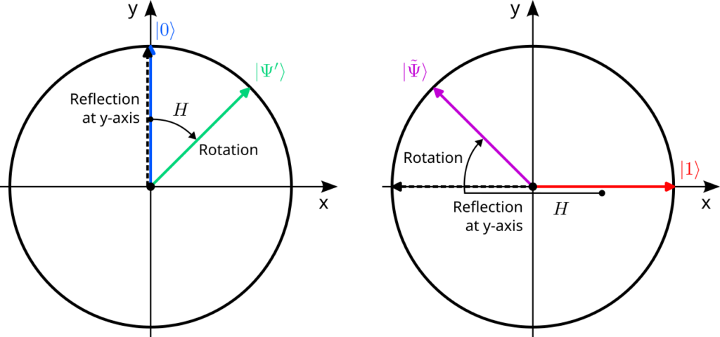
Note that the reflection at the y-axis does not affect the vector $\ket{0}$ so that it is only rotated by 45° clockwise. By contrast, the vector $\ket{1}$ is first reflected to $-\ket{1}$ and then rotated in the same way.
Many gates
The example above showed us an important property of gates in general: multiple gates can be combined to form new gates, and the “recipe” for their combination is simply their concatenation, i.e., one applies the first transformation (above: the reflection), then one applies the next transformation on the result of the first transformation (above: the rotation). The reason why this works is that the concatenation of two orthogonal maps again yields an orthogonal map. Intuitively this is clear: if two maps do not chance the length of vectors, their combination will neither. Let us collect all orthogonal maps in a set and call this set $O(2)$ (the “$O$” stands for “orthogonal” and the “$2$” tells us that our vectors are 2-dimensional), i.e., the elements of $O(2)$ are orthogonal linear maps. This may look weird at first, but the concept of sets in mathematics is very general: sets can contain numbers — but also more complicated objects like maps.
The set $O(2)$ has three very important properties; the possibility to “multiply” its elements by concatenating maps is one of them. Second, it contains a special “do nothing” map called identity which is simply the rotation by 0°. Lastly, for every orthogonal map you can find another orthogonal map, called its inverse, that “undoes” the action of the first one. A clockwise rotation by 45°, for example, can be undone by a counterclockwise rotation by the same angle. Reflections are their own inverse because reflecting twice at the same axis does nothing. A set with these three properties is called a group. The theory of groups — group theory — is an extremely important and rich field of mathematics, with applications in almost every field of physics. For example, the systematic classification of all possible crystal lattices is based on group theory, the three fundamental forces described by the Standard Model of particle physics (the electromagnetic, weak, and strong force) correspond to three specific groups, and the “Lorentz transformations” of Einstein’s theory of relativity are also described by a group. Groups are everywhere in physics!
The specific group $O(2)$ that contains all transformations of a single qubit is called the orthogonal group, so we can state in mathematical parlance:
The transformations of a single qubit form the orthogonal group $O(2)$.
Let us demonstrate the concatenation of gates again with the Hadamard gate. We start with a geometrical argument and then verify the outcome with abstract algebra. Our goal is to concatenate the Hadamard gate with itself, i.e., to apply it twice to the $\ket{0}$ state:$$
\ket{0}\;\xrightarrow{\;H\;}\;\ket{\Psi’}\;\xrightarrow{\;H\;}\;\ket{\Psi^{\prime\prime}}
$$Since the Hadamard gate is simply a reflection at the y-axis, followed by a clockwise rotation by 45°, we can compute the effect of this concatenation graphically:
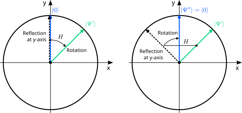
Note how the second application leads us back to where we started, $\ket{\Psi^{\prime\prime}}=\ket{0}$. You can check that this is not a special feature of our initial state $\ket{0}$: you always end up with the original vector after applying the Hadamard gate twice! In the language of group theory, the Hadamard gate $H$ is its own inverse transformation. We should check this hypothesis algebraically. So let us start with an arbitrary quantum state and apply the Hadamard gate twice, according to the “linearity rule” discussed previously:$$
\begin{aligned}
\ket{\Psi}=\alpha\ket{0}+\beta\ket{1}
\;&\xrightarrow{\; H \;}\;
\alpha\left(\frac{1}{\sqrt{2}}\ket{0}+\frac{1}{\sqrt{2}}\ket{1}\right)
+\beta\left(\frac{1}{\sqrt{2}}\ket{0}-\frac{1}{\sqrt{2}}\ket{1}\right)
\\[1em]
&\phantom{\;\xrightarrow{\; H \;}\;}=
\frac{\alpha+\beta}{\sqrt{2}}\ket{0}+\frac{\alpha-\beta}{\sqrt{2}}\ket{1}
\\[1em]
\;&\xrightarrow{\; H \;}\;
\frac{\alpha+\beta}{\sqrt{2}}\left(\frac{1}{\sqrt{2}}\ket{0}+\frac{1}{\sqrt{2}}\ket{1}\right)
+\frac{\alpha-\beta}{\sqrt{2}}\left(\frac{1}{\sqrt{2}}\ket{0}-\frac{1}{\sqrt{2}}\ket{1}\right)
\\[1em]
&\phantom{\;\xrightarrow{\; H \;}\;}=
\alpha\ket{0}+\beta\ket{1}=\ket{\Psi}
\end{aligned}
$$This proves that for every initial state $\ket{\Psi}$, applying the Hadamard gate twice leads us back to the same state $\ket{\Psi}$.
More generally, the calculation illustrates that the application of two (or more) concatenated gates on a state is no rocket science. One applies the gates one after another according to the rules of linear maps discussed earlier. After each application, it is convenient to use the rules of vector algebra to simplify the linear combination until every basis state ($\ket{0}$ and $\ket{1}$) occurs only once in the sum. That’s it.
The concatenation of many quantum gates on many qubits to implement a specific target transformation is what quantum computing is all about. Such a sequence of quantum gates is called a quantum algorithm, the quantum analog of a program that runs on a classical computer. But because quantum computers are only useful if they can manipulate many qubits, we should briefly discuss how gates operate on such states.
- Quantum gates can be composed by concatenating their actions.
- The set of all single-qubit gates forms a mathematical structure know as the orthogonal group.
- Groups are important structures used in many fields of physics. Groups have the important property that all their elements have an inverse element that undoes their action.
- The Hadamard gate can be illustrated as the concatenation of a reflection about the y-axis and a clockwise rotation by 45°.
- The Hadamard gate is its own inverse: Applying the Hadamard gate twice restores the original quantum state.
Beware:
Not all gates are their own inverse transformations. This is actually a rather rare property. The Hadamard gate is therefore an exception and not the rule. Consider rotations by some angle $\vartheta$, for example; can you explain for which angles $\vartheta$ rotations are their own inverse and for which not?
Many qubits
Remember that quantum states of $N$ qubits are simply normalized vectors in a $2^N$-dimensional vector space $\mathbb{R}^{(2^N)}$. They can be written as linear combination of the basis vectors $\ket{x_1x_2\dots x_N}$ where each $x_i$ is either $0$ or $1$ and describes the state of the qubit with index $i=1,\dots,N$. If one can define orthogonal linear maps for two-dimensional vectors, it shouldn’t be surprising that one can do the same thing for $2^N$-dimensional vectors. Hence there is a orthogonal group $O(2^N)$ for every $N$ that contains all allowed (= length preserving) quantum gates on $N$ qubits. For $N=1$ qubit, we get the orthogonal group on two-dimensional vectors back: $O(2^1)=O(2)$. As discussed before, we cannot visualize the states for $N>1$ qubits because we cannot imagine spaces of four dimensions and more. In particular, we cannot visualize quantum gates on such states, although they are still rotations (and reflections), but now in a very high dimensional space. But again, the abstract formalism of linear algebra remains a useful tool as it is applicable to vectors in any dimension.
To define a quantum gate $U$ on $N$ qubits, we must provide a list of transformations for all $2^N$ basis states $\ket{x_1x_2\dots x_N}$. Since each of these can be mapped to a linear combination with $2^N$ amplitudes, there are in total $2^N\times 2^N=2^{2N}$ real numbers $U_{ij}$ needed to specify the gate. These numbers must again fulfill a collection of constraints to ensure that all normalized vectors remain normalized after a transformation. Remember that the four numbers $U_{00},U_{01},U_{10},U_{11}$ of a single-qubit gate had to fulfill three equations. It turns out that for a general $U$ on $N$ qubits there are $2^N+2^N(2^N-1)/2$ such equations that must be fulfilled to make $U$ an orthogonal transformation. Here we will not discuss these constraints any further but demonstrate with two examples how quantum gates can be applied to many qubit states (we promise you that they fulfill the constraints and describe proper quantum gates!).
The Hadamard gate
Let us start again with the Hadamard gate and consider a setup of $N=2$ qubits. We introduced the Hadamard gate as a single-qubit gate, and this is still true if our system consists of two qubits. But now we have to decide on which of the two qubits we want to apply it! So strictly speaking, there are now two Hadamard gates, let us call them $H_1$ and $H_2$, where the index tells us on which of the two qubits the gate operates. Let us focus on $H_1$. Because the system consists of two qubits, there are four basis states,$$
\ket{00},\;\ket{01},\;\ket{10},\;\ket{11},
$$and any quantum gate on this system is defined by how it transforms these four states. This is also true for gates that operate only on a single qubit! The reason is that in quantum mechanics we cannot “split off” the state of one qubit and treat it separately; there is only the quantum state of all qubits combined, given as a linear combination of the four basis states above. The question is therefore what a “single-qubit gate” actually means in this context? Well, it means that the transformation rules of the basis states only depend on the configuration of the qubit on which it operates, the configurations of all other qubits are simply copied along:$$
\begin{aligned}
\ket{00}\;&\xrightarrow{\;H_1\;}\;\frac{1}{\sqrt{2}}\ket{00}+\frac{1}{\sqrt{2}}\ket{10}\\[1em]
\ket{01}\;&\xrightarrow{\;H_1\;}\;\frac{1}{\sqrt{2}}\ket{01}+\frac{1}{\sqrt{2}}\ket{11}\\[1em]
\ket{10}\;&\xrightarrow{\;H_1\;}\;\frac{1}{\sqrt{2}}\ket{00}-\frac{1}{\sqrt{2}}\ket{10}\\[1em]
\ket{11}\;&\xrightarrow{\;H_1\;}\;\frac{1}{\sqrt{2}}\ket{01}-\frac{1}{\sqrt{2}}\ket{11}
\end{aligned}
$$Note how the second row is a copy of the first row, except that the second qubit is flipped everywhere; similarly, the fourth row is a copy of the third with a flipped second qubit. You can imagine deleting the second qubit in all four transformation rules and you would recover the transformation rules of the Hadamard gate that we introduced previously for a single qubit (only that each rule would be duplicated). This property tells us that $H_1$ is a quantum gate that transforms only the first qubit: the transformation neither cares what the state of the second qubit is, nor does it change its state.
Can you write down the transformation rules for $H_2$?
Solution
The transformation rules for the Hadamard gate $H_2$ that operates on the second qubit are:$$
\begin{aligned}
\ket{00}\;&\xrightarrow{\;H_2\;}\;\frac{1}{\sqrt{2}}\ket{00}+\frac{1}{\sqrt{2}}\ket{01}\\[1em]
\ket{01}\;&\xrightarrow{\;H_2\;}\;\frac{1}{\sqrt{2}}\ket{00}-\frac{1}{\sqrt{2}}\ket{01}\\[1em]
\ket{10}\;&\xrightarrow{\;H_2\;}\;\frac{1}{\sqrt{2}}\ket{10}+\frac{1}{\sqrt{2}}\ket{11}\\[1em]
\ket{11}\;&\xrightarrow{\;H_2\;}\;\frac{1}{\sqrt{2}}\ket{10}-\frac{1}{\sqrt{2}}\ket{11}
\end{aligned}
$$In this case, the state of the first qubit is ignored and never changed.
The Controlled-NOT gate
Of course there are also gates that take into account the configurations of both qubits (and potentially change these configurations). Such gates are called multi-qubit gates in general and two-qubit gates if they operate on exactly two qubits. A particularly important two-qubit gate is the Controlled-NOT gate $\mathrm{CNOT}$ (the abbreviation “$\mathrm{CNOT}$” is the symbol for the gate and plays the same role has “$H$” for the Hadamard gate). In contast to the Hadamard gate, the Controlled-NOT gate does not produce superpositions; its job is to flip one qubit if and only if the other qubit is in state $\ket{1}$. The qubit that is flipped is called the target qubit, and the qubit that controls whether this flip occurs is called the control qubit. We can indicate this by indices: $\mathrm{CNOT}_{i,j}$ means that we use qubit $i$ as control and qubit $j$ as target. The transformation rules for a system of $N=2$ qubits read for $\mathrm{CNOT}_{1,2}$:$$
\begin{aligned}
\ket{00}\;&\xrightarrow{\;\mathrm{CNOT}_{1,2}\;}\;\ket{00}\\[1em]
\ket{01}\;&\xrightarrow{\;\mathrm{CNOT}_{1,2}\;}\;\ket{01}\\[1em]
\ket{10}\;&\xrightarrow{\;\mathrm{CNOT}_{1,2}\;}\;\ket{11}\\[1em]
\ket{11}\;&\xrightarrow{\;\mathrm{CNOT}_{1,2}\;}\;\ket{10}
\end{aligned}
$$Note how the state of the second qubit is toggled from $0$ to $1$ and back only in states where the first qubit is $1$; the state of the first qubit is not changed at all.
Can you write down the rules for $\mathrm{CNOT}_{2,1}$, i.e., the Controlled-NOT gate with the second qubit as control and the first one as target?
Solution
The transformation rules for the Controlled-NOT gate $\mathrm{CNOT}_{2,1}$ are:$$
\begin{aligned}
\ket{00}\;&\xrightarrow{\;\mathrm{CNOT}_{2,1}\;}\;\ket{00}\\[1em]
\ket{01}\;&\xrightarrow{\;\mathrm{CNOT}_{2,1}\;}\;\ket{11}\\[1em]
\ket{10}\;&\xrightarrow{\;\mathrm{CNOT}_{2,1}\;}\;\ket{10}\\[1em]
\ket{11}\;&\xrightarrow{\;\mathrm{CNOT}_{2,1}\;}\;\ket{01}
\end{aligned}
$$
- Quantum gates on many qubits are orthogonal maps (rotations and reflections) in a high-dimensional vector space.
- For $N$ qubits, a quantum gate is specified by the transformation rules of the $2^N$ basis states.
- Single-qubit gates like the Hadmard gates must be labeled by an index to indicate on which qubit it is applied.
- The transformation rules of single-qubit gates take into account and modify only the configuration of the qubit that they are applied to.
- Gates that take into account (and potentially change) the configurations of multiple qubits are kown as multi-qubit gates.
- The Controlled-NOT gate is an important example of a two-qubit gate. It flips the state of one qubit (the target) if and only if the state of another qubit (the control) is $\ket{1}$.
Many gates & many qubits:
A simple quantum algorithm
As a last example, let us construct a simple quantum algorithm on two qubits with a fascinating output (you’ll see!). Our goal is to concatenate the Hadmard gate $H_1$ on the first qubit with the Controlled-NOT gate $\mathrm{CNOT}_{1,2}$. This concatenation is some strange rotation and/or reflection in $O(2^2)=O(4)$ which transforms vectors in a four dimensional space. Luckily, with the powerful mathematical formalism of linear algebra in our toolbelt, there is no reason to be scared of high-dimensional spaces that we cannot imagine. So let us apply our knowledge and calculate the quantum state we obtain if we apply this gate sequence to the (very boring) initial state $\ket{\Psi_0}=\ket{00}$.
We start with the Hadamard gate on the first qubit:$$
\begin{aligned}
\ket{\Psi_0}=\ket{00}\;&\xrightarrow{\;H_1\;}\;\frac{1}{\sqrt{2}}\ket{00}+\frac{1}{\sqrt{2}}\ket{10}=\ket{\Psi_1}
\end{aligned}
$$Now we apply the Controlled-NOT gate on this state with the first qubit as control and the second as target:$$
\begin{aligned}
\ket{\Psi_1}\;&\xrightarrow{\;\mathrm{CNOT}_{1,2}\;}\;\frac{1}{\sqrt{2}}\ket{00}+\frac{1}{\sqrt{2}}\ket{11}=\ket{\Psi_2}
\end{aligned}
$$
Note how the second state in the linear combination transformed from $\ket{10}$ to $\ket{11}$. The state $\ket{\Psi_2}$ is so important that it has not one but two names: $\ket{\Psi_2}$ is known as a Bell state or an EPR pair.
So what? Where is the “fascinating output” that we promised? To cherish the strange properties of the Bell state $\ket{\Psi_2}$, we should measure it. Remember that so far we only transformed the state, we didn’t measure the qubits and no collapse of the quantum state occured. Let’s see what the Born rule tells us if we perform a measurement:$$
\ket{\Psi_2}=\frac{1}{\sqrt{2}}\ket{00}+\frac{1}{\sqrt{2}}\ket{11}
\;\xrightarrow{\;\text{Measurement}\;}\;
\ket{\Psi_3}=\begin{cases}
\ket{00} &\text{with}\;p_0=0.5\\
\ket{01} &\text{with}\; p_1=0\\
\ket{10} &\text{with}\; p_2=0\\
\ket{11} &\text{with}\; p_3=0.5\\
\end{cases}
$$Ok. So we observe only two possible outcomes, both with equal probability: $\ket{00}$, where both qubits are in state $0$, or $\ket{11}$ where both are in state $1$; we never observe an outcome where the two qubits are in different states.
But isn’t that strange? Imagine you prepare the Bell state in your laboratory on Earth (using our algorithm above), and then, before measuring, you send one of the two qubits with a spaceship to Mars (you hide both qubits in sealed boxes so that no measurement occurs). Then you open your box on Earth, and, simultaneously, an astronout opens the box on Mars, thereby perfoming a measurement of the qubits. Above we computed that the qubits on Earth and Mars will always be measured in the same random state! As if there was a hidden communication link between them to synchronize their random measurement outcomes, as if they where somehow … entangled. Indeed, the Bell state $\ket{\Psi_2}$ is the prime example of a quantum state with entanglement, the most notorious feature of quantum mechanics.
By the way, what would you find if you omit the Controlled-NOT gate from our algorithm above and only apply the single-qubit Hadamard gate $H_1$? Are there any signs of a “hidden communication link” in the probabilities for measurement outcomes?
Solution
Without the Controlled-NOT gate, we would measure the state $\ket{\Psi_1}$. The Born rule yields:$$
\ket{\Psi_1}=\frac{1}{\sqrt{2}}\ket{00}+\frac{1}{\sqrt{2}}\ket{10}
\;\xrightarrow{\;\text{Measurement}\;}\;
\ket{\Psi_3}=\begin{cases}
\ket{00} &\text{with}\;p_0=0.5\\
\ket{01} &\text{with}\; p_1=0\\
\ket{10} &\text{with}\; p_2=0.5\\
\ket{11} &\text{with}\; p_3=0\\
\end{cases}
$$Again there are only two possible outcomes, both with the same probabilities: $\ket{00}$ and $\ket{10}$. But these are not surprising at all! The first qubit (on Earth) behaves like a random number generator and spits out $0$ and $1$ with equal probability, while the second qubit (on Mars) doesn’t care: it is always is in state $0$.
We learn that the single-qubit Hadmard gate alone is not enough to produce entanglement. The two-qubit Controlled-NOT gate was absolutely crucial! One can show that this is a general mathematical fact: Quantum algorithms with only single-qubit gates never produce entangled states. To produce entanglement, multi-qubit gates like $\mathrm{CNOT}$ are an essential ingredient.
- Concatenations of many gates on many qubits are called quantum algorithms.
- A simple quantum algorithm is the application of a Hadamard gate, followed by a Controlled-NOT gate. The algorithm produces a so called Bell state.
- In a Bell state the two qubits are said to be entangled because measuring one of the qubits determines the measurement outcome of the other qubit.
- Entanglement can only be produced by multi-qubit gates. Single-qubit gates alone are not sufficient.
Entanglement
Now you know what the famous entanglement in quantum mechanics is! You learned even how to produce it with a quantum algorithm. That there seems to be a “hidden communication link” that synchronizes the two qubits instantaneously (in particular: faster than the speed of light!) was disliked by Albert Einstein so much that he referred to it as a “spooky action at a distance” — or at least so the story goes. Historically, the quote goes back to a 1947 letter by Einstein to Max Born (the one with the Born rule); he writes:
I cannot make a case for my attitude in physics which you
Albert Einstein to Max Born, March 3, 1947
would consider at all reasonable. I admit, of course, that there
is a considerable amount of validity in the statistical approach
which you were the first to recognise [..]. I cannot seriously
believe in it because the theory cannot be reconciled with the
idea that physics should represent a reality in time and space,
free from spooky actions at a distance. I am, however, not yet
firmly convinced that it can really be achieved with a continuous
field theory […].
In the letter, Einstein doesn’t mention the term “entanglement” at all (the term has been coined by Erwin Schrödinger more than 10 years earlier). His distress seems to stem from the collapse of the wavefunction that comes along with Born’s statistical approach to the measurement process. Remember that according to the Born rule, the quantum state is updated instantaneously to match the measurement outcome. In our thought experiment above, this update affects the common quantum state of both particles, irrespective of their distance. It is this instantaneous change of a non-local entity (the quantum state) that Einstein was at odds with because it heralds the downfall of local realism. “Local realism” is what Einstein means with “[…] the idea that physics should represent a reality in time and space“, i.e., the state of the world is completely specified at any point in time by local pieces of information. Intuitively, we are all like Einstein (local realists, that is) because the world we perceive in our everyday lives can be modeled in this way. It is actually hard to imagine what a world that is not locally realistic would be like.
Hence it may be discomforting to hear that most modern physisticst are convinced that our world is not locally realistic. This is indeed a consequence of entanglement, but not of the thought experiment we contrived above. When we discussed the measurement results of the two entangled qubits on Earth and Mars, we tricked you into believing that something “strange” is going on. After all, entanglement is supposed to be one of the strangest effects in quantum mechanics, right?! But imagine the following (classical) experiment: Put a blue and a red ball into box that can be separated into two boxes with a slider in the middle. Shake the box and ensure that one ball landed in each half of the box (do this without opening the box by checking that the weight of the box is balanced). Now close the slider and split the box into two sealed boxes, each containing a single ball. One of the boxes again is sent to Mars, one is left untouched in your laboratory. When you open the box, you find a red or a blue ball with equal probability, just like the qubit. But in the same moment, you know with certainty what an astronout on Mars will find in their box! If you find a blue ball, they will find a red one (and vice versa). Is there a “hidden communication link” between the two balls to make the ball on Mars red when yours is blue? Of course not, this is ridiculous! The experiment just illustrates the concept of correlations, and correlations have nothing to do with quantum physics. Our classical world is full of objects that are far apart but “know” things about each other: When you and your friend have the same pencil case and, after school, you rush home to find that you accidentally swapped the cases, you immediately know that your friend currently misses her pen. You didn’t have to call her to know this. You gained information about your friends current experience without any exchange of information, instantaneously! But this is neither surprising, nor “spooky”, and certainly does not violate the theory of relativity, according to which information is not allowed to travel faster than the speed of light. The correlation between your two pencil cases has been established locally (when you swapped them at school), just like the correlation between the two balls has been established locally (when you prepared the box on Earth). Similarly, the observation that the two qubits of our entangled quantum state always have the same value is another example of a correlation that has been setup locally (it is impossible to apply a Controlled-NOT gate on two qubits that are far apart). This implies in particular that quantum entanglement does not violate Einstein’s theory of relativity:
Entanglement cannot be used to send information faster than light!
We discuss this in more detail in our tutorials where you can implement the entanglement-producing algorithm above on our simulator of a quantum computer.
- Entanglement is a special form of correlation in quantum mechanics.
- The correlations of entangled states are stronger than any classical, locally realistic theory allows. This is the statement of Bell’s theorem.
- Local realism is a view, advocated by Albert Einstein, according to which the state of the world is completely specified at any point in time by local pieces of information.
- Experimental Bell tests showed that the predictions of quantum mechanics are correct. This means that our world is not locally realistic.
- Entanglement cannot be used to send information faster than light. Quantum mechanics is consistent with Einstein’s special theory of relativity.
One of the postulates of Einstein’s special theory of relativity is that the speed of light in vacuum $c$ is the upper limit at which any signal carrying information can travel through space. For the consistency of quantum mechanics with the special theory of relativity, it is therefore crucial that entangled qubits cannot be used for instantaneous information transmission. Luckily, this impossibility is implied by the postulates of quantum mechanics, a fact formalized by the no-communication theorem.
But if entanglement is “just” a type of correlation, why is there so much hype about it among physicists? The reason is that it is a surprisingly strong type of correlation (called quantum correlation) that cannot be explained by theories that adhere to Einstein’s tenet of local realism. This “strength” is already hidden in the entangled Bell state that we prepared with our quantum algorithm above; however, a more sophisticated measurement procedure is needed to unveil it (which is a bit too technical for this tutorial). The upshot is that one can show and quantify mathematically that the correlations of the Bell state cannot be realized by classical systems that are described by local pieces of information (like the color of the two balls or the contents of the two pencil cases). This mathematical statement is known as Bell’s Theorem, an inequality for correlations that is violated by quantum mechanics. Experiments known as Bell tests have demonstrated beyond any reasonable doubt that the Bell inequality is indeed violated, and the predictions of quantum mechanics are correct. This implies that the locally realistic worldview advocated by Einstein does not match reality. It is this result that makes entanglement and quantum mechanics “weird”, or at least unintuitive. In a nutshell:
The “strangeness” of entanglement is not the existence of correlations, but their strength which cannot be explained by locally realistic theories.
Note that Bell’s Theorem was published in 1964 and the first Bell test was performed in 1972 by John Clauser (for which he was awarded the 2022 Nobel Prize in Physics, jointly with Alain Aspect and Anton Zeilinger), long after Einstein died in 1955. It would be fascinating to hear what Einstein had to say about these results.
Relative and Global Signs
There is one last thing about quantum states that we swept under the rug: The role played by the sign of amplitudes. Remember that we introduced the amplitudes $\alpha$ and $\beta$ of the single qubit quantum state$$
\ket{\Psi}=\alpha\ket{0}+\beta\ket{1}\quad\text{with}\quad \alpha^2+\beta^2=1
$$ as real numbers, i.e., they are allowed to be negative. But when we compute the probabilities for measurement outcomes with the Born rule, the signs drop out because we square the amplitudes. This begs the question whether we actually need negative amplitudes at all. Do we loose anything if $\alpha \geq 0$ and $\beta \geq 0$, or, equivalently, if $\ket{\Psi}$ points only into the first quadrant of the xy-plane? The answer to this question is remarkably subtle.
Let us consider exemplarily the following two states which both have at least one negative amplitude:$$
\ket{\Psi_1}=-1\cdot\ket{0}\quad\text{and}\quad \ket{\Psi_2}=\frac{1}{\sqrt{2}}\cdot\ket{0}-\frac{1}{\sqrt{2}}\cdot\ket{1}
$$If we measure a qubit in state $\ket{\Psi_1}$, the Born rule tells us that the outcome $\ket{0}$ is observed with probabability $p_0=\alpha^2=(-1)^2=1$, i.e., the state collapses deterministically into $\ket{0}$. By contrast, a qubit in state $\ket{\Psi_2}$ is found in $\ket{0}$ with probability $p_0=\alpha^2=(1/\sqrt{2})^2=0.5$ and in state $\ket{1}$ with probability $p_1=\beta^2=(-1/\sqrt{2})^2=0.5$. So far so good, but what about the very similar states$$
\ket{\Psi’_1}=+1\cdot\ket{0}\quad\text{and}\quad \ket{\Psi’_2}=\frac{1}{\sqrt{2}}\cdot\ket{0}+\frac{1}{\sqrt{2}}\cdot\ket{1}
$$where we flipped all negative signs to positive ones? If you apply the Born rule again, you will find the exact same probabilities as for the states above (this is not surprising since the signs drop out when squaring the amplitudes). But if the probabilities for measurement outcomes are the same for the states with and without a prime, how can we distinguish them? Aren’t they then the same state? Not so fast! In the previous section you learned that before measuring we can also manipulate the qubit by applying gates. So the most general “operation” that we can perform on a qubit is the combination of some gate followed by a measurement. We should therefore ask whether there is any gate that allows us to tell the vectors with and without prime apart if we apply the gate before measuring the qubit. If there is such a gate, the vectors describe clearly different physical states—this difference is only a bit harder to detect. But if there is no such gate, we would have to accept that there can be different vectors that describe the same physical state; in particular, the terms “vector” and “(quantum) state” would describe not exactly the same thing!
- That amplitudes can be negative is an important feature of quantum states.
- Pairs of quantum states that yield the same probability distribution for measurement outcomes can yield different measurement results if one applies a quantum gate prior to the measurement.
- Signs that affect only some of the amplitudes are called relative signs. Vectors that differ by relative signs can be experimentally distinguished and correspond to distinct quantum states.
- Pairs of quantum states which differ only in a global sign (that affects all amplitudes) cannot be distinguished by any combination of gates and measurements. Such vectors describe the same quantum state. We say that quantum states are equivalence classes of vectors.
For a start, let us take the Hadamard gate $H$ defined in the section above and apply it to our four states. For the superposition $\ket{\Psi_2}$ with a negative amplitude we find$$
\begin{aligned}
\ket{\Psi_2}\;\xrightarrow{\;H\;}\;
&=\frac{1}{\sqrt{2}}\left(\frac{1}{\sqrt{2}}\ket{0}+\frac{1}{\sqrt{2}}\ket{1}\right)-\frac{1}{\sqrt{2}}\left(\frac{1}{\sqrt{2}}\ket{0}-\frac{1}{\sqrt{2}}\ket{1}\right)\\[1em]
&=\left(\frac{1}{2}-\frac{1}{2}\right)\ket{0}+\left(\frac{1}{2}+\frac{1}{2}\right)\ket{1}\\[1em]
&=\ket{1}
\end{aligned}
$$Measuring this state yields the outcome $\ket{1}$ with certainty ($p_1=\beta^2=1$). By contrast, for the state $\ket{\Psi’_2}$ with flipped sign we find$$
\begin{aligned}
\ket{\Psi’_2}\;\xrightarrow{\;H\;}\;
&=\frac{1}{\sqrt{2}}\left(\frac{1}{\sqrt{2}}\ket{0}+\frac{1}{\sqrt{2}}\ket{1}\right)+\frac{1}{\sqrt{2}}\left(\frac{1}{\sqrt{2}}\ket{0}-\frac{1}{\sqrt{2}}\ket{1}\right)\\[1em]
&=\left(\frac{1}{2}+\frac{1}{2}\right)\ket{0}+\left(\frac{1}{2}-\frac{1}{2}\right)\ket{1}\\[1em]
&=\ket{0}
\end{aligned}
$$and we measure the outcome $\ket{0}$ with certainty ($p’_0=\alpha^2=1$). So we can tell these two states apart! The trick is to apply a Hadamard gate before we measure. In particular, this means that the vectors $\ket{\Psi_2}$ and $\ket{\Psi’_2}$ really describe different physical states of the qubit, and that the minus sign of the second amplitude in $\ket{\Psi_2}$ is important. We can conclude:
The fact that probability amplitudes can become negative is important.
In particular, quantum states are more than mere probability distributions.
The phenomenon of interference in quantum mechanics can only be explained with the negativity of probability amplitudes. The fact that amplitudes can be positive or negative allows for cancellations that supress the probability for certain measurement outcomes. For example, the famous double-slit experiment demonstrates the interference of the wave function of single particles (like electrons); in regions where the probability to find particles vanishes, positive and negative amplitudes cancel. The role played by interference in quantum computing is explored in one of our tutorials.
While this statement is true, it is missing a very important “but”. To understand why, let us focus on the other pair or of states $\ket{\Psi_1}$ and $\ket{\Psi’_1}$. If we again apply the Hadamard gate to both of them, we find$$
\begin{aligned}
\ket{\Psi_1}=(-1)\cdot\ket{0}\;&\xrightarrow{\;H\;}\;-\frac{1}{\sqrt{2}}\ket{0}-\frac{1}{\sqrt{2}}\ket{1}\,,\\
\ket{\Psi’_1}=(+1)\cdot\ket{0}\;&\xrightarrow{\;H\;}\;+\frac{1}{\sqrt{2}}\ket{0}+\frac{1}{\sqrt{2}}\ket{1}\,.
\end{aligned}
$$The Born rule tells us that in both cases the outcomes $\ket{0}$ and $\ket{1}$ occur with equal probability:$$\begin{aligned}
p_0&=(-1/\sqrt{2})^2=0.5=(1/\sqrt{2})^2=p’_0\,,\\
p_1&=(-1/\sqrt{2})^2=0.5=(1/\sqrt{2})^2=p’_1\,.
\end{aligned}
$$So here the Hadamard gate does not help us to tell the two states appart because $p_0=p’_0$ and $p_1=p’_1$. This result, of course, does not prove that they cannot be distinguished; maybe there is another gate that can make them distinguishable? We could start to try randomly gates and hope that we find a useful one. A more frutiful approach is to not fix a gate at all but to apply the general form discussed in the previous section. For the state without prime this results in$$
\ket{\Psi_1}=(-1)\cdot\ket{0}\;\xrightarrow{\;U\;}\;(-1)\cdot (U_{00}\ket{0}+U_{01}\ket{1})
$$and we measure $\ket{0}$ with probability $p_0=(-U_{00})^2=U_{00}^2$ and $\ket{1}$ with probability $p_1=(-U_{01})^2=U_{01}^2$. By contrast, the sign-flipped state with a prime is transformed to$$
\ket{\Psi’_1}=(+1)\cdot\ket{0}\;\xrightarrow{\;U\;}\;(+1)\cdot (U_{00}\ket{0}+U_{01}\ket{1})
$$ and we find the probabilities $p’_0=(+U_{00})^2=U_{00}^2$ and $p’_1=(+U_{01})^2=U_{01}^2$ respectively. But they are the same! More precisely:$$
p_0=p’_0\quad\text{and}\quad p_1=p’_1
$$Most importantly, this result does not depend on the gate $U$. So no matter which gate we apply before measuring, we can never tell the states $\ket{\Psi_1}$ and $\ket{\Psi’_1}$ apart! What is going on? Didn’t we just say that signs are important?
Yes, they are; but only if they are relative signs, i.e., signs that affect some but not all amplitudes of a linear combination. By contrast, global signs affect all amplitudes in the same way and these signs cannot be measured. Our two examples illustrate this difference, which is formally reflected in the following two (in)equalities:$$
\ket{\Psi_1}=(-1)\cdot\ket{\Psi’_1}
\quad\text{but}\quad
\ket{\Psi_2}\neq (-1)\cdot\ket{\Psi’_2}
$$The relation between $\ket{\Psi_1}$ and $\ket{\Psi’_1}$ qualifies the minus sign in $\ket{\Psi_1}$ as a global sign. The sign in $\ket{\Psi_2}$, however, is a relative sign that affects only one of the two amplitudes: If you try to pull the $(-1)$ in front of $\ket{\Psi_2}$, the vector that is left is no longer $\ket{\Psi’_2}$ but some other vector.
What we just showed above for the special case of $\ket{\Psi_1}$ and $\ket{\Psi’_1}$ is true for all pairs of vectors that are related by a global sign:$$
\ket{\Psi}=(-1)\cdot\ket{\Psi’}
$$Such vectors cannot be distinguished by any sequence of gates and measurements that you can cook up. This means that they represent the same physical state! Thus we have been sloppy so far in using the term “vector” and “state” interchangeably. The true quantum states are more like “sets of vectors” that are related by global signs: $\{\ket{\Psi},-\ket{\Psi}\}$. The vectors in one such set then act like “lables” that all denote the same quantum state. Mathematicians love this kind of construction. They even have a name for the sets: they call them equivalence classes. Let us summarize what we have learned so far:
Vectors that differ in relative signs describe different quantum states.
Vectors that differ in global signs describe the same quantum state.
Therefore:
Quantum states are equivalence classes of of the form $\{\pm\ket{\Psi}\}$.
The fact that global signs do not influcence the outcomes of arbitrary sequences of gates and measurements is a direct consequence of the linearity of quantum gates. The example illustrates this: the global minus sign in $\ket{\Psi_1}$ is simply “carried along” and only affects the sign (but not the absolute value) of the final probabilty amplitudes. After squaring, these signs drop out and the probabilities remain unaffected.
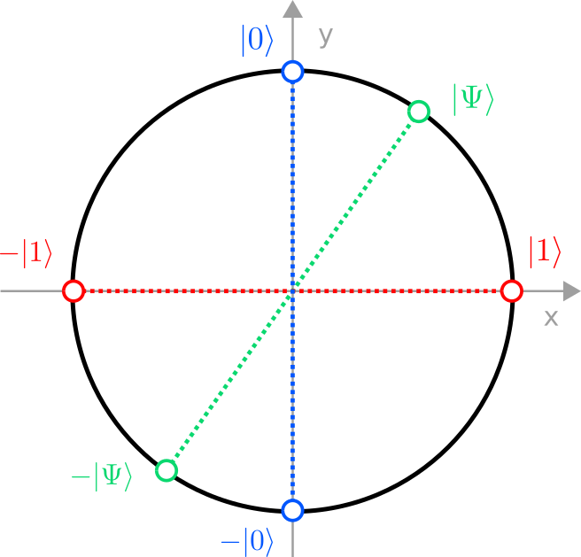
The Bloch Circle
What a bummer! It seemed that we can visualize the state space of a single qubit nicely by our circle of unit vectors, but now we have to concede that this is not exactly right: Since the antipodes on the circle correspond to the equivalence classes $\{\pm\ket{\Psi}\}$, our description is redundant, i.e., for every quantum state there are two points on the circle that describe or “label” it. This is quite unintuitive — what we really want is a visualization of the true “space of quantum states” (= state space). The points in such a space should somehow correspond to equivalence classes $\{\pm\ket{\Psi}\}$ rather than vectors! Mathematicians call spaces that are made of equivalence classes quotient spaces. The particular quotient space that describes our single qubit quantum states is called the real projective line, it’s symbol is $\mathbb{R}P^1$. Let us construct it!
We would like to find a space where every point can be mapped one-to-one to a pair of antipodes $\{\pm\ket{\Psi}\}$ on the unit circle. The trick is to realize that these two antipodes both lie on a infinite line (called a ray) through the origin:
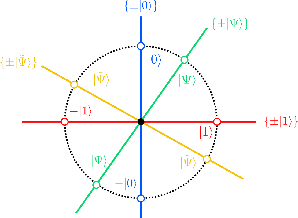
This means that there is a one-to-one correspondence between rays and quantum states (If I give you a ray, you know which quantum state $\{\pm\ket{\Psi}\}$ I mean; conversely, if you want to tell me a quantum state $\{\pm\ket{\Psi}\}$, you can simply give me the ray on which the two vectors lie). The set of all rays through the origin is called a ray space or projective space. In some books on quantum mechanics you will therefore read that “the state space of a qubit is a ray space” and “quantum states are rays” .
This is all very nice, but let’s be honest: imagining a space made out of “rays” is somewhat strange. Intuitively, spaces should be made out of “points” of some sort. Is there a way to construct a space where every point corresponds to exactly one ray through the origin (and therefore to one quantum state)? Yes! Just attach an infinite real line $\mathbb{R}$ to the top of the circle and associate every ray with its intersection on this line:
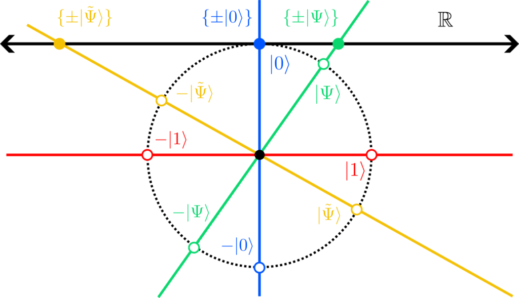
Every ray defines one point on this line, and, vice versa, every point on the line defines a ray. Perfect! Wait, every ray? No, every ray but the horizontal one that corresponds to the quantum state $\{\pm\ket{1}\}$. Because it is parallel to $\mathbb{R}$, it never intersects the line. We are therefore missing a single intersection that represents $\{\pm\ket{1}\}$. There is a recurring scheme in mathematics: When you are missing something, just add it! Remember that we are constructing a new space with the goal to represent the unintuitive space of rays. We are therefore allowed to modify the real line $\mathbb{R}$ to fix our problem. Our fix is simple: we add a single point called “$\infty$” and declare that one approaches this point if one travels further and further either to the right or the left on the line:
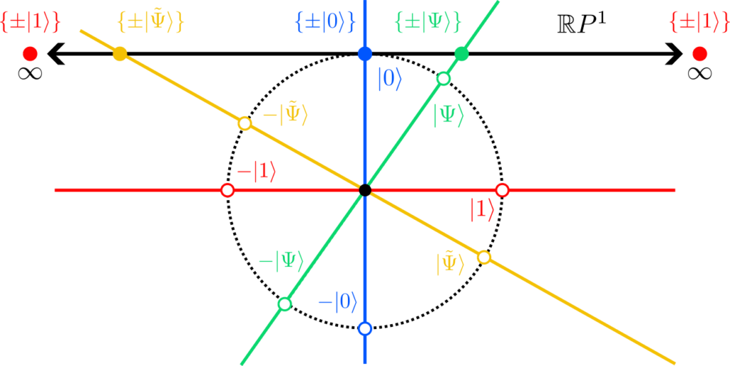
Note that there is really only one point “$\infty$” that shows up twice in the figure! Mathematicians call this procedure one-point compactification of $\mathbb{R}$, and the resulting space is again called the real projective line $\mathbb{R}P^1$. Why? Well, what happens if you start from a vertical ray and observe its intersection with $\mathbb{R}$ as you slowly rotate towards the horizontal? Depending on the direction in which you rotate, the intersection quickly travels either to “plus infinity” or “minus infinity” on the line $\mathbb{R}$. But we just declared that the point you approach in either direction is the new point called “$\infty$”. So “$\infty$” is exactly the missing intersection of the horizontal ray that encodes the state $\{\pm\ket{1}\}$! The one-point compactified real line therefore is the space we were looking for: Every point corresponds to exactly one ray through the origin. It therefore makes sense to identify the one-point compactified real line with the projective line $\mathbb{R}P^1$, i.e., the state space of a single qubit. The state $\{\pm\ket{1}\}$ is then represented by the single (!) point “$\infty$” at infinity.
Great, you say, we got rid of the rays but now we have a point “$\infty$” at infinity with the strange property that one approaches it if one travels either to the left or to the right on the real line. But is that really so strange? After all, it doesn’t matter whether you fly along earth’s equator for 20.000 km to the east or to the west, you will eventually end up at the same point. Just like the equator, which looks very straight if you are standing on it, the one-point compactification $\mathbb{R}P^1$ is a circle! It just happens to have “infinite” radius and therefore appears as a perfectly straight line. But remember that we set out to find a space with a one-to-one correspondence between points and quantum states, so the “geometric form” or “size” of the space shouldn’t really bother us. Let us then “shrink” the real projective line to a unit circle where the point “$\infty$” is no longer strange and distinct from the others and simply becomes the “south pole”:
- In mathematics, spaces made out of equivalence classes are called quotient spaces.
- An example is the space of the equivalence classes that describes all possible quantum states of a single qubit. This particular quotient space is called the real projective line.
- The real projective line can be illustrated as a unit circle, known as the “Bloch circle”.
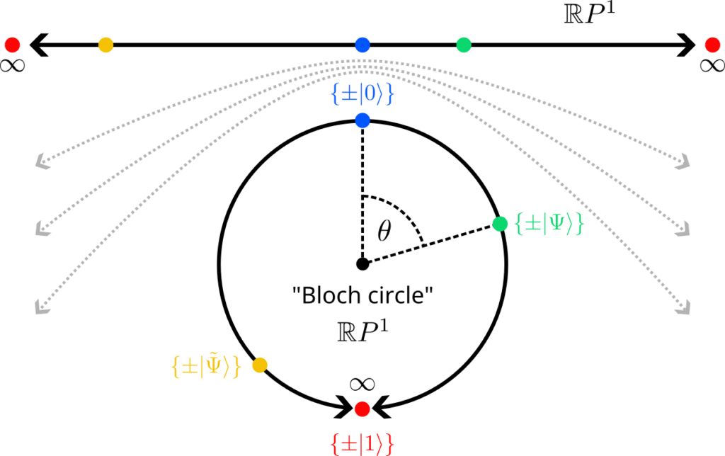
Finally! The state space of a single qubit is the real projective line $\mathbb{R}P^1$, which we can illustrate as a circle. On this circle, every point corresponds to a unique quantum state $\{\pm\ket{\Psi}\}$, which is the equivalence class of two antipodal unit vectors. But beware: This new circle is different from our original unit circle. To make this distinction clear, let us call $\mathbb{R}P^1$ the Bloch circle (we explain below where this name comes from). For example, the state $\{\pm\ket{1}\}$ sits now on the “south pole” of the Bloch circle and is no longer separated by a 90° angle from the state $\{\pm\ket{0}\}$ at the “north pole”. So do not mistakenly take the points on the Bloch circle as vectors pointing in this direction! The vectors in $\{\pm\ket{0}\}$ and $\{\pm\ket{1}\}$ are still orthogonal, although it doesn’t look like it on the Bloch circle. The points on the Bloch circle are equivalence classes $\{\pm\ket{\Psi}\}$, and if you want to know how the vectors $\pm\ket{\Psi}$ look like, you would have to undo all the transformations we discussed above. Luckily, there is a much simpler way to translate points on the Bloch circle back to vectors.
Since we cannot directly linear combine equivalence classes $\{\pm\ket{\Psi}\}$, we have to resort to unit vectors $\ket{\Psi}$ as “labels” of these classes. Our goal is therefore to find a parametrization of $\ket{\Psi}$ such that no equivalence class is represented by two redundant vectors, i.e., it should be impossible to construct both $+\ket{\Psi}$ and $-\ket{\Psi}$ with our parametrization. If you have a look at the Bloch circle above, it seems reasonable to use the angle $\theta$ to parametrize the states on the circle. We want $\theta=0$ to yield $\{\pm\ket{0}\}$, represented by, say, $\ket{0}$, and $\theta=\pi$ to yield $\{\pm\ket{1}\}$, represented by, say $\ket{1}$. This can easily be achieved by the linear combination
$$
\ket{\Psi}=\cos\left(\frac{\theta}{2}\right)\ket{0}+\sin\left(\frac{\theta}{2}\right)\ket{1}
\quad\text{for}\quad -\pi<\theta\leq \pi\,.
$$Note that in comparison to our previous parametrization at the beginning of this tutorial, the angles are now divided by 2 so that $\theta = \pi$ yields $\ket{1}$ and not $-\ket{0}$ (which would be redundant!). Indeed, you can check that adding $\pi$ to any angle $\theta$ (which corresponds to the antipode on the Bloch circle) yields$$
\begin{aligned}
\ket{\Psi’}&=\cos\left(\frac{\theta+\pi}{2}\right)\ket{0}+\sin\left(\frac{\theta+\pi}{2}\right)\ket{1}\\
&=-\sin\left(\frac{\theta}{2}\right)\ket{0}+\cos\left(\frac{\theta}{2}\right)\ket{1}
\neq (-1)\cdot\ket{\Psi}
\end{aligned}
$$which is no longer related to the original vector by a global phase. Our Bloch circle parametrization therefore produces physically different states for different angles $\theta$, and hence correctly visualizes the state space of a single qubit.
Beware:
You may wonder: How is it possible that we start from a unit circle, merge all points with their antipodes into one point, and again end up with a unit circle (the Bloch circle)? Shouldn’t the new circle be “half as big”? Well, no. Which of the two intervals $[0,1]$ and $[0,2]$ do you think contains more points? Well, they contain exactly the same (infinite) number of points! You can easily check this with the function $f(x)=2x$ which assigns every point in $[0,1]$ a unique point in $[0,2]$ and vice versa. “Infinity” can be an unintuitive concept!
Beware:
Despite being aware of these mathematical concepts, physicists (including us) are not used to think in terms of “projective spaces” and “rays” because it is not a very useful concept for what we do. It is also not a very intuitive concept, you might add, and most physicists would agree. Hence we actually prefer to stick with the picture of vectors and just keep in mind that global signs are not important. Physicists also tend to be sloppy in their nomenclature: We don’t distinguish between vectors and states, i.e., we refer to the vector $\ket{\Psi}$ as a “quantum state” while being fully aware that $(-1)\cdot\ket{\Psi}$ is the same quantum state. In this sense, we do not make a distinction between the equivalence classes and the things in it. While this is mathematically not quite correct, it turns out to be a convenient mindset to apply quantum mechanics as a tool. Notwithstanding, the Bloch sphere (see below) is widely used in quantum physics, altough its relation to projective spaces is mostly ignored.
If you followed the tutorial up to this point, you can give yourself a pat on the back. By now you have a basic understanding of the formalism of quantum mechanics that is almost on par with the knowledge of an undergrad student of physics after their first course in quantum mechanics. In paticular, you are equipped with all the tools needed to understand a variety of simple quantum algorithms that can be run on a quantum computer.

One last thing …
There is a last confession to be made: You should never tell a physicist that the state space of a qubit is the Bloch circle. In the best-case scenario, they look at you with blank eyes; in the worst case, they snigger. The reason is that the true state space of a single qubit is not described by a circle but by a sphere:
The state space of a single qubit is the Bloch sphere.
The reason goes back right to the beginning of this tutorial where we argued that the amplitudes $\alpha$ and $\beta$ of quantum states are real numbers $\mathbb{R}$. This is a simplification needed to make the tutorial accessible with the mathematical tools taught at school.
In reality, probability amplitudes are complex numbers $\mathbb{C}$.
Complex numbers can be thought of as a “superset” of real numbers (equivalently: $\mathbb{R}$ is a subset of $\mathbb{C}$). The framework we discussed remains valid, only that it can be extened to complex numbers. For instance, the orthogonal group $O(2)$ that describes the single-qubit gates can be extended to its complex counterpart, the unitary group $U(2)$. The state space is also not the real projective line $\mathbb{R}P^1$ but the complex projective line $\mathbb{C}P^1$ since the equivalence classes not only contain two vectors $\{\pm\ket{\Psi}\}$ with different signs but infinitely many vectors $\{e^{i\varphi}\ket{\Psi}\}$ with different phases $\varphi$ (think of phases as generalization of signs). A similar construction then produces a sphere instead of a circle. If you want to learn about complex numbers and understand what $\mathbb{C}P^1$ has to do with a sphere, you should read the optional section below.
Apart from that:
- The amplitudes of quantum states are actually complex numbers.
- Complex numbers are a superset of real numbers. All equations we wrote down remain valid in the full formalism but can be extended to complex numbers.
- The full set of single-qubit gates is the unitary group.
- The state space of a single qubit is the complex projective line and can be illustrated by the Bloch sphere.
after the physicist Felix Bloch.
You are now ready to program a quantum computer!
The complete picture (Optional)

Ⓒ2023 Tutorial by Nicolai Lang, Institute for Theoretical Physics III, University of Stuttgart