Coherence and Decoherence

Useful qubits must remain coherent to be useful for quantum computation. Qubits can become incoherent through a process called decoherence; when this happens, they can no longer be used for quantum algorithms. Thus coherent qubits are desirable, and decoherence is to be prevented at all costs. The degradation process of decoherence is triggered by “accidental measurements”, i.e., when information about the qubit leaks into the environment. Here we illustrate with a simple example how one can check whether a qubit remained coherent, and how the process of decoherence can be modeled with our quantum circuit simulator.

In a previous tutorial we discussed the effect of interference, i.e., the cancellation of positive and negative amplitudes in superposition states. We illustrated this phenomenon with the following simple quantum circuit:

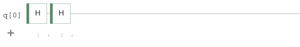
When we applied the Hadamard gate twice, we found that the second one undoes the superposition created by the first one so that we measured the qubit in its initial state $\ket{0}$ with certainty.

This exact cancellation of amplitudes only worked because in between the two Hadamard gates the qubit state was not altered. If it were modified only slightly, the cancellation would no longer be perfect and the interference would fail. This failure of interference would be indicated by a non-zero probability to find the qubit in state $\ket{1}$ at the end. We can therefore use interference experiments to check whether a qubit leaked information or whether it remained unperturbed. If the probability to find $\ket{1}$ after the second Hadamard gate is zero, we say that the qubit remained coherent between the two Hadamard gates.

To represent the waiting time between the two gates, let us add a few identity gates $I$ between them:

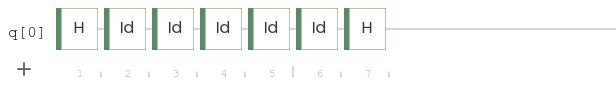
Because the identity gates are “do nothing operations”, the histogram should not change by this modification, i.e., the interference remains perfect and the qubit coherent during the algorithm.

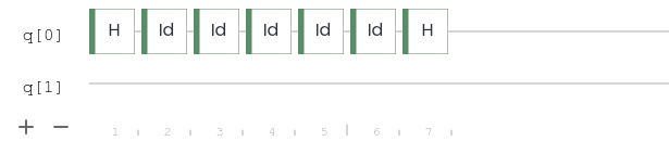
Now we would like to simulate a process where information about the qubit leaks into the environment during the interference experiment, i.e., between the two Hadamard gates. To this end, we use an additional qubit to represent the environment, so click  +  to add another qubit. We are not interested in the measurement outcome of this qubit as it is a stand-in for the environment — and we typically do not know what the environment “knows”. Disposable qubits like this that are only used “internally” to make an algorithm work are called ancillas. We refer to this ancilla as environment henceforth to distinguish it from the qubit used for the interference experiment (which we simply call the qubit).

If you let the algorithm

run, the result will not change, of course. The qubit still remains coherent because there is no coupling between the qubit and the environment. This is the dream of every quantum engineer: the qubits you care about are completely decoupled from the environment and remain coherent for as long as you want. Unfortunately, it is impossible to achieve this in practice. If you wait long enough, some information will eventually leak out (for example by a random photon bouncing of your qubit).

To simulate this, let us connect the qubit with a Controlled-NOT gate to the environment. Since we want the environment to gain information, but not change the state of the qubit, make sure that the control of the Controlled-NOT gate (the $\bullet$ symbol) is on the qubit, and the target (the $\oplus$ symbol) is on the ancilla:

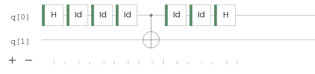
Now the ancilla is flipped from $\ket{0}$ to $\ket{1}$ if and only if our qubit is in state $\ket{1}$. The state of the qubit is not changed. So the environment gains knowledge about the state of the qubit during the interference experiment.

Observe the histogram of this circuit and compare it to the previous ones. You can also try to change the position of the Controlled-NOT gate and observe what happens. What is the probability to find the qubit in state $\ket{1}$?