Quantum Algorithms & Quantum Circuits

Writing quantum algorithms

A quantum computer is a machine that can manipulate the quantum state of many qubits in a controlled way. The output of the computation is the measurement of all qubits at the end of this transformation. Because quantum mechanics is a probabilistic theory, many such runs (called shots) are necessary to average the outcomes and compute the probabilities to measure certain states.

A single shot can be described as follows:
$$
\underbrace{\ket{\Psi_\mathrm{initial}}=\ket{0\dots 0}}_{\text{Initialization}}\;
\underbrace{\xrightarrow{\qquad U=U_M\,\cdots\,U_2\,U_1\qquad }}_{\text{Quantum algorithm}}
\;\ket{\Psi_\mathrm{final}}
\;\xrightarrow{\;\text{Measure all qubis}\;}\;
\underbrace{\begin{cases}
\ket{0\dots 0}&?\\
\ket{0\dots 1} &?\\
&\vdots \\
\ket{1\dots 1} &?
\end{cases}}_{\text{Output}}
$$There are three crucial steps to perform a shot:

1. Initialization of all qubits in the state $\ket{\Psi_\mathrm{initial}}=\ket{0\dots 0}$.
2. Transformation of the initial quantum state by applying a sequence of quantum gates $U=U_M\,\cdots\,U_2\,U_1$ according to a prescribed “quantum program” or quantum algorithm. This produces the final state $\ket{\Psi_\mathrm{final}}$.
3. Measurement of all qubits and output of the result $\ket{q_N,\dots,q_1}$ with $q_i\in\{0,1\}$.

These steps are then repeated many times to approximate the probabilities for the observed qubit states by averaging the results of all shots.

The crucial step is of course the application of the transformation $U$. “Programming a quantum computer” simply means to specify which $U$ should be applied. To make the specification of $U$ easier, a set of primitive gates $\{X,Y,Z,H,\dots\}$ that act either on one, two, or three qubits is provided by the quantum computing platform. The job of the “quantum programmer” is to combine these primitive gates to implement $U$:$$
U=U_M\,\cdots\,U_2\,U_1\quad\text{with}\quad U_i\in\{X,Y,Z,H,\dots\}
$$A specific sequence of primitve gates $(U_1,U_2,\dots,U_M)$ is called a quantum algorithm. In the notation above, primitive gates are applied from right to left, i.e., starting with $U_1$ and ending wth $U_M$. $M$ is the total number of applied gates, it determines the runtime of the quantum algorithm.

A quantum circuit is a graphical representation of a quantum algorithm $U=U_M\,\cdots\,U_2\,U_1$ where qubits are represented by horizontal lines and time flows from left to right:

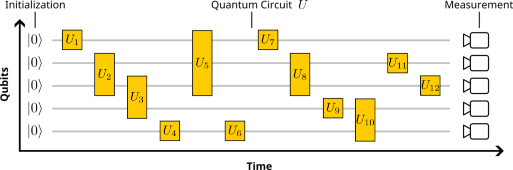
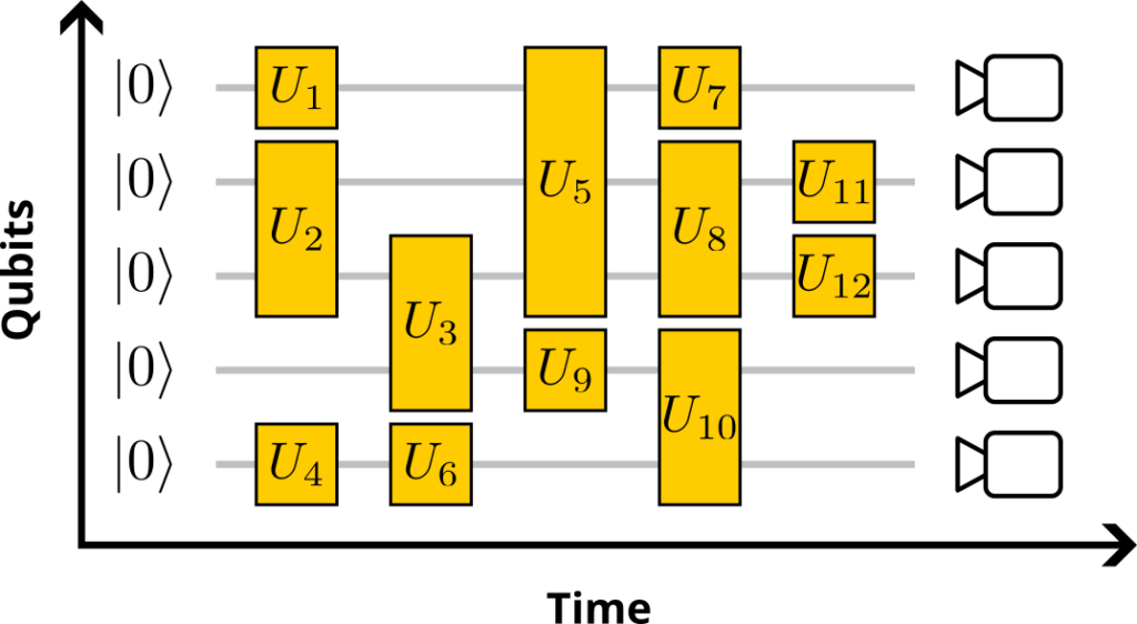
The primitive gates $U_i$ are represented by boxes that cover the lines of the qubits that the gates operate on. Gates that act on a single qubit are represented by squares, gates that act on two adjacent qubits by rectangles etc. The left boundary of the circuit corresponds to the initial state $\ket{\Psi_\mathrm{initial}}=\ket{0\dots 0}$, the right boundary to the final state $\ket{\Psi_\mathrm{final}}$ and the subsequent measurement of all qubits. Gates that operate on different qubits (= disjoint boxes) can be applied in parallel so that the circuit above can be compactified as follows:

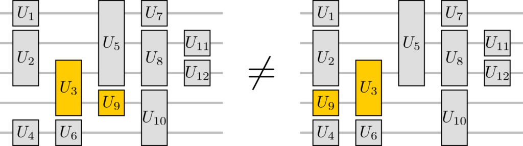
However, it is crucial that the sequence of gates matters (they do not commute). So the following circuits are not equivalent in general and produce different final states (and measurement outcomes):

The Quantum Circuit Simulator

Here we describe how our quantum circuit simulator works step by step:

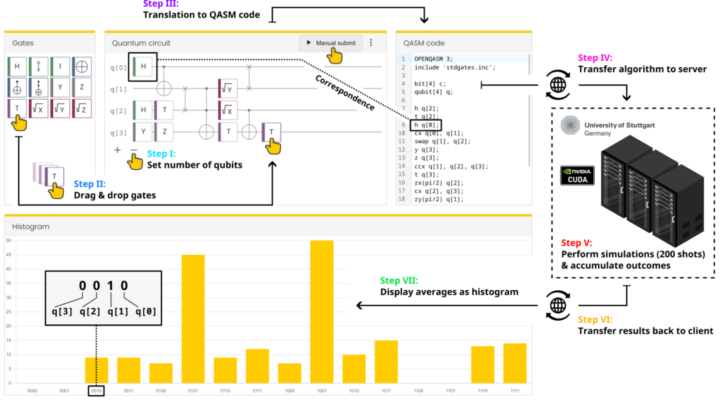
Step I
Use the + and - buttons in the Quantum circuit box to set the number of qubits (1–10 qubits are possible). The qubits are labeled as q[i] with index i=0,1,...,N-1 for N qubits (in informatics, indices typically start from 0 and not 1).

Step II
Use your mouse to drag quantum gates from the Gates box into the Quantum circuit box. Drop the gate on the horizontal line that corresponds to the qubit that the gate should be applied to. You can insert gates before other gates by “squeezing” them in gaps between gates. To delete gates, grab them and pull them out of the quantum circuit.

Step III
Whenever you change the quantum circuit, the quantum circuit simulator automatically translates the circuit into an equivalent OpenQASM code representation (shown in the QASM code box).

Step IV
After the OpenQASM code has been updated, it is automatically sent to our QRydDemo API at the University of Stuttgart and queued in the job list of our classical simulator. You can also manually submit a new job by clicking the Manual submit button. This is useful to observe the statistical fluctuations of the measurement outcomes.

Step V
Our simulator of a quantum computer executes your quantum circuit 200 times and accumulates the measurement outcomes. The simulator runs on dedicated graphics cards to accelerate the computations. When our quantum computer is up and running, this simulation can be replaced by a quantum computation on a real quantum computer.

Note: To simulate quantum algorithms on up to 10 qubits, it is not necessary to use dedicated hardware like graphics cards. These simulations could be performed by your local computer (even in your browser). However, we use this simulation pipeline & hardware also productively to simulate up to 32 qubits and optimize our gate protocols. It was then straightforward to connect the quantum circuit simulator to this pipeline, so that you automatically profit from improvements of our simulators.

Step VI
The accumulated measurement results are sent back to the quantum circuit simulator in your browser.

Step VII
The results are displayed in the Histogram box of the quantum circuit simulator. The y-axis shows the number of shots that resulted in a specific qubit configuration after measurement (all bars therefore add up to 200). On the x-axis the $2^N$ possible measurement outcomes are shown (for $N$ qubits). For example, the label 0010=q[3]q[2]q[1]q[0] corresponds to the measured state $\ket{q_3q_2q_1q_0}=\ket{0010}$.

Gates

Here we list and define all primitive gates that are currently supported by the quantum circuit simulator. Gates marked as “native” are directly supported by the QRydDemo quantum computing platform. Gates that are not native are automatically translated into native gates when the quantum algorithm is compiled on our servers.

Note: The native two-qubit gate of the QRydDemo platform is a Controlled-Phase gate which is currently not directly available in the quantum circuit simulator (it will be in an upcoming version). The multi-qubit gates that are available are automatically translated into Controlled-Phase gates by our compiler.

Name	Symbol	# Qubits	Definition	Native?
Identity		1	$I=\begin{pmatrix}1&0\\0&1\end{pmatrix}$	Yes
Pauli-X		1	$X=\begin{pmatrix}0&1\\1&0\end{pmatrix}$	Yes
Pauli-Y		1	$Y=\begin{pmatrix}0&-i\\i&0\end{pmatrix}$	Yes
Pauli-Z		1	$Z=\begin{pmatrix}1&0\\0&-1\end{pmatrix}$	Yes
Sqrt-X		1	$\sqrt{-iX}=\frac{1}{\sqrt{2}}\begin{pmatrix}1&-i\\-i&1\end{pmatrix}$	Yes
Sqrt-Y		1	$\sqrt{-iY}=\frac{1}{\sqrt{2}}\begin{pmatrix}1&-1\\1&1\end{pmatrix}$	Yes
Sqrt-Z (Phase)		1	$S=\sqrt{Z}=\begin{pmatrix}1&0\\0&i\end{pmatrix}$	Yes
$\pi/8$ (T)		1	$T=\begin{pmatrix}1&0\\0&e^{i\pi/4}\end{pmatrix}$	Yes
Hadamard		1	$H=\frac{1}{\sqrt{2}}\begin{pmatrix}1&1\\1&-1\end{pmatrix}$	No
Controlled-NOT (CNOT)		2	$\mathrm{CNOT}=\begin{pmatrix}1&0&0&0\\0&1&0&0\\0&0&0&1\\0&0&1&0\end{pmatrix}$	No
Swap		2	$\mathrm{SWAP}=\begin{pmatrix}1&0&0&0\\0&0&1&0\\0&1&0&0\\0&0&0&1\end{pmatrix}$	No
Toffoli (CCNOT)		3	$\mathrm{Toff}=\begin{pmatrix} 1 & 0 & 0 & 0 & 0 & 0 & 0 & 0 \\ 0 & 1 & 0 & 0 & 0 & 0 & 0 & 0 \\ 0 & 0 & 1 & 0 & 0 & 0 & 0 & 0 \\ 0 & 0 & 0 & 1 & 0 & 0 & 0 & 0 \\ 0 & 0 & 0 & 0 & 1 & 0 & 0 & 0 \\ 0 & 0 & 0 & 0 & 0 & 1 & 0 & 0 \\ 0 & 0 & 0 & 0 & 0 & 0 & 0 & 1 \\ 0 & 0 & 0 & 0 & 0 & 0 & 1 & 0 \end{pmatrix}$	No

Ⓒ2023 Tutorial by Nicolai Lang, Institute for Theoretical Physics III, University of Stuttgart