Your first quantum algorithm: The Deutsch-Jozsa Algorithm
For our first simulations, configure the simulator with a single qubit so that there is only one line in the quantum circuit.
Simulation 1: Doing nothing
Without any gates, the transformation applied by the quantum computer is simply:
$$
\ket{\Psi_\mathrm{initial}}=\ket{0}
\;\xrightarrow{\; I \;}\;
\underbrace{1}_{\alpha}\ket{0}+\underbrace{0}_{\beta}\ket{1}
=\ket{\Psi_\mathrm{final}}
\;\xrightarrow{\mathrm{Measure}}\;
\begin{cases}\ket{0}&:\,p_0=1.0\\\ket{1}&:\,p_1=0.0\end{cases}
$$Here $I$ denotes the “do nothing operation” called identity. At the end the final state is measured and yields the result $\ket{0}$ with probability $p_0=1$. So in this example, the measurement outcome is indeed deterministic (but also very boring).
- A machine that follows the rules of quantum mechanics (a quantum computer) can solve certain problems much faster than a classical computer.
- We only know of a handful of problems where this applies (the most famous being integer factorization on which the RSA cryptosystem is based). Designing quantum algorithms is hard!
The Good
- Quantum computers can exponentially speedup the simulation of quantum mechanics itself!
The Bad
- Quantum computers do not speedup algorithms because they “try every possible solution in parallel”.
If this would be true, they would speedup essentially every algorithm – which they don’t. In particular, quantum computers will not be useful to speedup computer games (sorry)! - Quantum computers are not expected to solve NP hard problems (like “travelling salesman”) exponentially faster.
- There is no mathematical proof that quantum computers are faster than classical computers at all, but there is strong evidence that this is the case.
The No-Cloning Theorem and the SWAP gate
On a classical computer you can copy bits as much as you like. For instance, the bits that make up the content of this webpage have been copied to your computer from our server — it would be really stupid if they could not be copied but only moved because then only one person at a time could look at the webpage. Nonetheless, this is exactly how quantum information works! The mathematical fact that one cannot copy a qubit is known as No-Cloning Theorem.
The No-Cloning Theorem
Without any gates, the transformation applied by the quantum computer is simply:
$$
\ket{\Psi_\mathrm{initial}}=\ket{0}
\;\xrightarrow{\; I \;}\;
\underbrace{1}_{\alpha}\ket{0}+\underbrace{0}_{\beta}\ket{1}
=\ket{\Psi_\mathrm{final}}
\;\xrightarrow{\mathrm{Measure}}\;
\begin{cases}\ket{0}&:\,p_0=1.0\\\ket{1}&:\,p_1=0.0\end{cases}
$$Here $I$ denotes the “do nothing operation” called identity. At the end the final state is measured and yields the result $\ket{0}$ with probability $p_0=1$. So in this example, the measurement outcome is indeed deterministic (but also very boring).
- The unknown quantum state of a qubits cannot be copied reliably.
- This No-Cloning Theorem follows from the linearity of quantum mechanics. It is therefore baked into the defining properties of quantum mechanics. The impossibility to clone quantum information is not a “downside to be fixed”.
- This is a problem for correcting errors on qubits.
- However, it can also be exploited for quantum cryptography.
Coherence and Decoherence
Useful qubits must remain coherent for as long as possible. The goal of this tutorial is to understand what this means. Qubits can become incoherent through a process called decoherence; when this happens, they are useless for quantum computation. Thus coherent qubits are desirable, and decoherence is to be prevented at all costs. The degradation process of decoherence is triggered by “accidental measurements”, i.e., when information about the qubit leaks into the environment. Here we illustrate with a simple example how one can check whether a qubit remained coherent, and how the process of decoherence can be modeled with our quantum circuit simulator.
In the previous tutorial we discussed the effect of interference, i.e., the cancellation of positive and negative amplitudes in superposition states. We illustrated this phenomenon with the following simple quantum circuit:
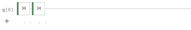
When we applied the Hadamard gate twice, we found that the second one undoes the superposition created by the first one so that we measured the qubit in its initial state $\ket{0}$ with certainty.
This exact cancellation of amplitudes only worked because in between the two Hadamard gates the qubit state was not altered. If it were modified only slightly, the cancellation would no longer be perfect and the interference would fail. This failure of interference would be indicated by a small but non-zero probability to find the qubit in state $\ket{1}$ at the end. We can therefore use interference experiments to check whether a qubit leaked information or whether it remained unperturbed. If the probability to find $\ket{1}$ after the second Hadamard gate is zero, we say that the qubit remained coherent between the two Hadamard gates.
To represent the waiting time between the two gates, let us add a few identity gates $I$ between them:
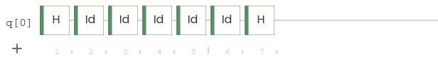
Because the identity gates are “do nothing operations”, the histogram should not change by this modification, i.e., the interference remains perfect and the qubit coherent during the algorithm.
Now we would like to simulate a process where information about the qubit leaks into the environment during our interference experiment, i.e., between the two Hadamard gates. To this end, we use an additional qubit to represent the environment, so click + to add another qubit. We are not interested in the measurement outcome of this qubit as it is a stand-in for the environment — and we typically do not know what the environment “knows”. Disposable qubits like this that are only used “internally” to make an algorithm work are called ancillas. We refer to this ancilla as environment henceforth to distinguish it from the qubit used for the interference experiment (which we simply call the qubit). If you let the algorithm
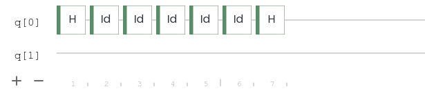
run, the result will not change, of course. The qubit still remains coherent because there is no coupling between the qubit and the environment. This is the dream of every quantum engineer: the qubits you care about are completely decoupled from the environment and remain coherent for as long as you want. Unfortunately, it is really hard to achieve this in practice. If you wait long enough, some information will eventually leak (for example by a random photon bouncing of your qubit). To simulate this, let us connect the qubit with a Controlled-NOT gate to the environment. Since we want the environment to gain information, but not change the state of the qubit, make sure that the control of the Controlled-NOT gate (the $\bullet$ symbol) is on the qubit, and the target (the $\oplus$ symbol) is on the ancilla:
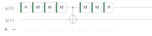
Now the ancilla is flipped from $\ket{0}$ to $\ket{1}$ if and only if our qubit is in state $\ket{1}$. The state of the qubit is not changed. So the environment gains knowledge about the state of the qubit during the interference experiment.
Observe the histogram and compare it to the previous ones. You can also try to change the position of the Controlled-NOT gate and observe what happens. What is the probability to find a state where the qubit is in state $\ket{1}$?
Explanation
The chance of finding the qubit in state $\ket{1}$ is given by the sum of the probabilities for the output state $\ket{0\underline 1}$ and $\ket{1\underline 1}$ because we do not care in which state the ancilla is measured (we underlined the state of the qubit q[0] which we used for the interference experiment). In probability theory, such a sum is called a marginal.
The important point is that there is now a 50% chance to find the qubit after the second Hadamard gate in state $\ket{1}$, a result that would be impossible if the qubit had not been coupled to the environment between the two Hadamard gates. This means that there is no interference anymore that cancels positive and negative amplitudes, i.e., the qubit lost its coherence — it decohered. The fascinating thing is that the measurement results for the qubit changed although the Controlled-NOT gate never flipped the qubit (remember that we used it as control, not as target!).
The maximal time one can wait between the two Hadamard gates without destroying the interference (equivalently: loosing the coherence) is an important number that quantifies the “quality” of a qubit and is called the coherence time. When building a quantum computer, it is important to make the coherence time of the qubits as long as possible (this is one of the experimentally most challenging obstacles when building a quantum computer). Typical coherence times on the QRydDemo platform are of the order 10 milliseconds.
You might think that this is not very long. This is correct, but “not very long” is a relative statement. Remember that the coherence time essentially measures how long a qubit remains usable for quantum computations. The important question is therefore whether the coherence time is long enough to apply all gates needed for a specific quantum algorithm. On our platform, the application of a gate takes roughly 100 nanoseconds. This means that in a perfect world, and with the above coherence time, we can execute quantum algorithms that comprise on the order of several hundreds gates. This is already not bad, but it is not nearly enough to unleash the full power of a quantum computer. So in the end it is true: The coherence times are not long enough! So we have to work harder to make them better, right?
There is a problem with this endeavor. The coherence time is determined by how well one can isolate a qubit (for us: an atom) from the environment. But we already use single atoms in vacuum. Yes, there are still photons flying around, but most of them are not relevant because they do not have the wavelength needed to read out the qubit. (Recall that to measure the qubits we have to illuminate the atoms with a laser of a specific wavelength, and this condition must also be met by the “environmental photons”, of course.) So while there is a bit of headroom to increase the coherence time of our qubits by shielding them even better, it is not enough to increase the decoherence times arbitrarily (e.g., into the range of seconds). The problem we encounter is so fundamental that the whole quantum computing endeavor seems doomed: one cannot decouple an atom perfectly from the rest of the universe, because even the vacuum is not empty! This is a result of the Standard Model of particle physics and know as vacuum energy or vacuum fluctuations. For our Strontium atoms, these fluctuations can cause a change of the qubit state no matter how well we shield the atom (we cannot remove the vacuum fluctuations from the vacuum because the laws of nature don’t allow this!). It is important to let that sink in. Our coherence times cannot be increased drastically because the laws of nature forbid it, not because our technologies are lacking improvements.
The complete picture (Optional)
The above picture of a qubit as two-dimensional vector of length one is almost correct. The only simplification was that the coefficients (the amplitudes) $\alpha$ and $\beta$ were taken to be real numbers $\mathbb{R}$, while in reality they are complex numbers $\mathbb{C}$. This makes the state space of a proper qubit harder (but not impossible) to visualize. None of the examples in this tutorial require this additional structure, so that you can skip this optional part if you like. (The complex number are essential for an efficient formulation of quantum mechanics, though.)
Complex Numbers
A complex number $\alpha$ can be written as$$
\alpha = \alpha_r+i\cdot \alpha_i
$$with real part $\alpha_r\in\mathbb{R}$ and imaginary part $\alpha_i\in\mathbb{R}$ (yes, the imaginary part is a real number!). The symbol “$i$” denotes the imaginary unit; it is formally defined by the property $i=\sqrt{-1}$ so that $i^2=-1$. The space of complex numbers is labeled by $\mathbb{C}$.
Calculations with complex numbers simply follow from the distributive and associative laws together with $i\cdot i =-1$. For example, adding two complex numbers yields$$
\alpha+\beta=(\alpha_r+i\cdot\alpha_i)+(\beta_r+i\cdot\beta_i)=\underbrace{(\alpha_r+\beta_r)}_{\gamma_r}+i\cdot\underbrace{(\alpha_i+\beta_i)}_{\gamma_i}=\gamma
$$and their product is$$
\alpha\cdot\beta=(\alpha_r+i\cdot\alpha_i)\cdot(\beta_r+i\cdot\beta_i)=\underbrace{(\alpha_r\beta_r-\alpha_i\beta_i)}_{\delta_r}+i\cdot\underbrace{(\alpha_r\beta_i+\alpha_i\beta_r)}_{\delta_i}=\delta\,.
$$Hence one can think of complex numbers as a generalization of real numbers with modified rules for multiplication and addition.
The cool thing about complex numbers is that every polynomial equation has a solution (mathematicians call this algebraically closed)! For example, the equation$$
x^2=-1
$$ has no solution in the real numbers, but it has two complex solutions: $x_1=+i$ and $x_2=-i$. For this and other reasons, both in mathematics and physics, complex numbers $\mathbb{C}$ are the “standard type” of numbers used for the description of many problems, just as the real numbers $\mathbb{R}$ are the “standard numbers” used in school.
- A qubit is a two-dimensional vector of length 1. It is not a classical bit that is in an unkown state 0 or 1.
- The components of the vector are called (probability) amplitudes and can be negative.
- Only the squares of the amplitudes are positive and are interpreted as the probabilities to measure the qubit in a particular state.
TODO
Qubits: Vectors with complex Amplitudes
Quantum mechanics is no exception. Therefore the most general quantum state of a qubit can be written as
$$
\ket{\Psi}=\alpha\ket{0}+\beta\ket{1}=\begin{pmatrix}\beta\\\alpha\end{pmatrix}
$$where the two amplitudes $\alpha,\beta\in\mathbb{C}$ are now complex numbers. You cannot visualize this vector as “pointing” in some direction in a two-dimensional space (the deeper reason for this is that complex numbers, unlike real numbers, cannot be ordered from small to large numbers). For example, where would you say the complex vector$$
\begin{pmatrix}i\\0\end{pmatrix}
$$ points to? (I have no clue.) This makes the true quantum states less intuitive than the simplified real ones from above, but not less rigorous – we can still do calculations with them!
The condition that the vector must have length 1 now reads$$
|\alpha|^2+|\beta|^2\stackrel{!}{=}1
$$ where $|\alpha|=\sqrt{\alpha_r^2+\alpha_i^2}$ is called the modulus (or absolute value) of the complex number $\alpha$. Note that $\alpha^2$ does note make sense in the above equation because we want this to be a positive real number (to interpret it as a probability); but for $\alpha=i$ we would get $\alpha^2=-1$, which we cannot read as a probability. By contrast, $|\alpha|^2=\alpha_r^2+\alpha_i^2=0+1^2=1$ is perfectly positive and real.
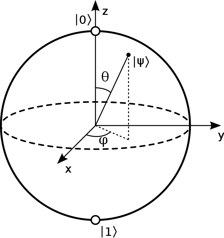
Do we gain anything by replacing real amplitudes with complex ones? The answer is yes: the space of possible states that a qubit can have becomes in some sense larger when using complex amplitudes. So we should expect that the different states of a qubit can no longer be visualized as a simple unit circle. They can, however, be visualized by a sphere of radius 1, the so called Bloch sphere. To understand how this is possible (it is not obvious!), we first have to state a beautiful equation called Euler’s formula:$$
e^{i\varphi}=\cos(\varphi)+i\cdot \sin(\varphi)
$$Here $\varphi\in\mathbb{R}$ is an arbitrary real number, $i$ is again the imaginary unit, $\sin$ and $\cos$ are the trigonometric functions, and $e=2.718\dots$ is a very special real number called Euler’s number (it shows up all over mathematics).
When following mathematical arguments like the ones that led us here, one can easily loose contact to reality and forget what we actually want to achieve. The use of complex amplitudes that gives rise to the Bloch sphere as the state space of a qubit is so far just a (beautiful) mathematical concept. But in the end we want to use mathematics to describe the actual qubits stored in the orbitals of the electrons in our atoms. Do we really need all this unintuitive complexity (pun intended) to describe their states? The clear answer is: Yes! We can change the states of our qubits in ways that cannot be described by real amplitudes. The states of our qubits really are described by points on the Bloch sphere, and not by points on a unit circle. This tells us a very important lesson: Complex numbers are not just inventions of mathematicans, they are, in some sense, the natural language needed to describe nature.
Simulation 2: Creating many entangled qubits
Make sure that the circuit simulator is setup with three qubits q[0], q[1], and q[2].
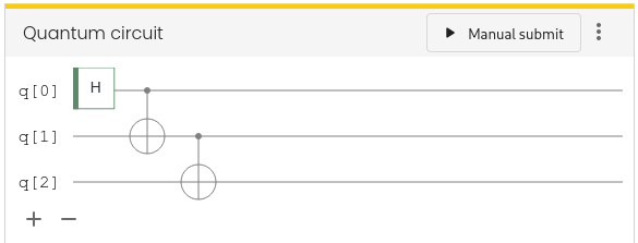
Can you construct a circuit on more than three qubits that entangles all of them in a GHZ state? Assume there is a chance of $p=0.01$ (1%) for each qubit to be accidentaly measured in the timespan of a second (for instance, by the environment). What is the probability that a GHZ state with $N=10$ qubits collapses in one second? What is the probability for $N=100$ qubits?
Explanation
TODO